Operations on images with BandMath and BandMathX
Simple calculus using BandMath
The BandMath application provides a simple and efficient way to perform pixel wise operations. It computes a band wise operation according to a user defined mathematical expression. The following code computes the absolute difference between first bands of two images.
otbcli_BandMath -il input_image_1 input_image_2
                -exp "abs(im1b1 - im2b1)"
                -out output_image
The naming convention “im[x]b[y]” designates the yth band of the xth input image.
The BandMath application embeds built-in operators and functions listed in muparser documentation thus allowing a vast choice of possible operations.
Advanced image operations using BandMathX
One limitation of the BandMath application is that it can only output mono-band images, because the mu-parser library only support scalar expressions. In contrast, the BandMathX application based on the mu-parserX library can output both mono and multi band images, and supports expressions containing scalars, vectors and matrices. The following code compute the difference between two images:
otbcli_BandMathX -il input_image_1 input_image_2
                -exp "im1 - im2"
                -out output_image
The output image produced by this application has the same number of bands as the input images, and each resulting band contains the difference between the corresponding bands in the input images.
Syntax: first elements
Variables and their descriptions:
| Variables | Type | Description |
|---|---|---|
| im1 | Vector | a pixel from first input, made of n components/bands (first image is indexed by 1) |
| im1bj | Scalar | jth component of a pixel from first input (first band is indexed by 1) |
| im1bjNkxp | Matrix | a neighborhood (”N”) of pixels of the jth component from first input, of size kxp |
| im1bjMini | Scalar | global statistic: minimum of the jth band from first input |
| im1bjMaxi | Scalar | global statistic: maximum of the jth band from first input |
| im1bjMean | Scalar | global statistic: mean of the jth band from first input |
| im1bjSum | Scalar | global statistic: sum of the jth band from first input |
| im1bjVar | Scalar | global statistic: variance of the jth band from first input |
| im1PhyX and im1PhyY | Scalar | spacing of first input in X and Y directions |
In addition, we also have the generic variables idxX and idxY that represent the indices of the current pixel (scalars).
Note that the use of a global statistics will automatically make the filter (or the application) request the largest possible regions from the concerned input images, without user intervention.
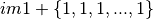
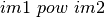
For instance, the following formula (addition of two pixels)

is correct only if the two first inputs have the same number of bands. In addition, the following formula is not consistent even if im1 represents a pixel of an image made of only one band:

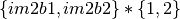
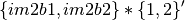
A scalar can’t be added to a vector. The right formula is instead (one can notice the way that muParserX allows vectors to be defined on the fly):

or
if im1 is made of n components.
On the other hand, the variable im1b1 for instance is represented as a scalar; so we have the following different possibilities:
Correct / incorrect expressions:
| Expression | Status |
|---|---|
| im1b1 + 1 | correct |
| {im1b1} + {1} | correct |
| im1b1 + {1} | incorrect |
| {im1b1} + 1 | incorrect |
| im1 + {im2b1,im2b2} | correct if im1 represents a pixel of two components (equivalent to im1 + im2) |
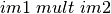
Similar remarks can be made for the multiplication/division; for instance, the following formula is incorrect:
whereas this one is correct:
or in more simple terms (and only if im2 contains two components):

Concerning division, this operation is not originally defined between two vectors (see next section New operators and functions).
Now, let’s go back to the first formula: this one specifies the addition of two images band to band. With muParserX lib, we can now define such operation with only one formula, instead of many formulas (as many as the number of bands). We call this new functionality the batch mode, which directly arises from the introduction of vectors within muParserX framework.
Operations using neighborhoods
Let’s say a few words about neighborhood variables. These variables are defined for each particular input, and for each particular band. The two last numbers, kxp, indicate the size of the neighborhood. All neighborhoods are centered: this means that k and p can only be odd numbers. Moreover, k represents the dimension in the x direction (number of columns), and p the dimension in the y direction (number of rows). For instance, im1b3N3x5 represents the following neighborhood:
| . | . | . |
|---|---|---|
| . | . | . |
| . | . | . |
| . | . | . |
| . | . | . |
For example, the following code subtract the mean value in a 3x3 neighborhood around each pixel to the pixel value, using the first band of the input image:
otbcli_BandMathX -il input_image_1 input_image_2
                -exp "im1b1 - mean(im1b1N3x3)"
                -out output_image
Fundamentally, a neighborhood is represented as a matrix inside the muParserX framework; so the remark about mathematically well-defined formulas still stands.
Operations involving bit manipulation
Sometimes, manipulating bits instead of real numbers is useful. For instance, multiple binary masks are sometime stored altogether in a mono-band integer image.
In order to manipulate bit, one need to convert its data into integer (because the data is read as floating point numbers). To do so, muParserX has a type conversions operator: (int). Prefixing your images with it will allow you to perform such operations.
- Example:
(int)im1b1 & 0b00000001(bitwise and)(int)im1b1 >> 1(right shift operator)
New operators and functions
In addition to the operators and functions available in muParserX (https://beltoforion.de/article.php?a=muparserx), new ones have been implemented within OTB. These ones can be divided into two categories:
- adaptation of existing operators/functions, that were not originally defined for vectors and matrices (for instance cos, sin, …). These new operators/ functions keep the original names to which we add the prefix “v” for vector (vcos, vsin, …) .
- truly new operators/functions.
Concerning the last category, here is a list of implemented operators or functions (they are all implemented in otbParserXPlugins.h/.cxx files OTB/Modules/Filtering/MathParserX):
Operators div and dv: The first operator allows the definition of an element-wise division of two vectors (and even matrices), provided that they have the same dimensions. The second one allows the definition of the division of a vector/matrix by a scalar (components are divided by the same unique value). For instance:

Operators mult and mlt: These operators are the duals of the previous ones. For instance:
Operators pow and pw: The first operator allows the definition of an element-wise exponentiation of two vectors (and even matrices), provided that they have the same dimensions. The second one allows the definition of the division of a vector/matrix by a scalar (components are exponentiated by the same unique value). For instance:

Note that the operator ’*’ could have been used instead of ’pw’. But ’pw’ is a little bit more permissive, and can tolerate a one-dimensional vector as the right operand.
Function bands: This function allows to select specific bands from an image, and/or to rearrange them in a new vector; for instance:
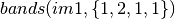
produces a vector of 4 components made of band 1, band 2, band 1 and band 1 values from the first input. Note that curly brackets must be used in order to select the desired band indices.
Function dotpr: This function allows the dot product between two vectors or matrices (actually in our case, a kernel and a neighborhood of pixels):
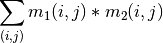
For instance:

is correct provided that kernel1 and im1b1N3x5 have the same dimensions.
Function mean: This function allows to compute the mean value of a given vector or neighborhood (the function can take as many inputs as needed; one mean value is computed per input). For instance:

Note: a limitation coming from muparserX itself makes it impossible to pass all those neighborhoods with a unique variable.
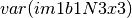
Function var: This function computes the variance of a given vector or neighborhood (the function can take as many inputs as needed; one var value is computed per input). For instance:
Function median: This function computes the median value of a given vector or neighborhood (the function can take as many inputs as needed; one median value is computed per input). For instance:
Function corr: This function computes the correlation between two vectors or matrices of the same dimensions (the function takes two inputs). For instance:

Function maj: This function computes the most represented element within a vector or a matrix (the function can take as many inputs as needed; one maj element value is computed per input). For instance:

Function vmin and vmax: These functions calculate the min or max value of a given vector or neighborhood (only one input, the output is a 1x1 matrix). For instance:

Function cat: This function concatenates the results of several expressions into a multidimensional vector, whatever their respective dimensions (the function can take as many inputs as needed). For instance:

Note: the user should prefer the use of semi-colons (;) when setting expressions, instead of directly use this function. The filter or the application will call the function ’cat’ automatically. For instance:

Function ndvi: This function implements the classical normalized difference vegetation index; it takes two inputs. For instance:
First argument is related to the visible red band, and the second one to the near-infrared band.
The table below summarizes the different functions and operators.
Functions and operators summary:
| Variables | Remark |
|---|---|
| ndvi | two inputs |
| bands | two inputs; length of second vector input gives the dimension of the output |
| dotptr | many inputs |
| cat | many inputs |
| mean | many inputs |
| var | many inputs |
| median | many inputs |
| maj | many inputs |
| corr | two inputs |
| div and dv | operators |
| mult and mlt | operators |
| pow and pw | operators |
| vnorm | adaptation of an existing function to vectors: one input |
| vabs | adaptation of an existing function to vectors: one input |
| vmin | adaptation of an existing function to vectors: one input |
| vmax | adaptation of an existing function to vectors: one input |
| vcos | adaptation of an existing function to vectors: one input |
| vsin | adaptation of an existing function to vectors: one input |
| vtan | adaptation of an existing function to vectors: one input |
| vtanh | adaptation of an existing function to vectors: one input |
| vsinh | adaptation of an existing function to vectors: one input |
| vcosh | adaptation of an existing function to vectors: one input |
| vlog | adaptation of an existing function to vectors: one input |
| vlog10 | adaptation of an existing function to vectors: one input |
| vexp | adaptation of an existing function to vectors: one input |
| vsqrt | adaptation of an existing function to vectors: one input |
| vect2scal | one dimensional vector to scalar |
Context and Constant
Thanks to the -incontext one can pass constant value to the application in order to use it in the expression. For the definition of constants, the following pattern must be observed: #type name value. For instance:
#F expo 1.1 #M kernel1 { 0.1 , 0.2 , 0.3 ; 0.4 , 0.5 , 0.6 ; 0.7 , 0.8 , 0.9 ; 1 , 1.1 , 1.2 ; 1.3 , 1.4 , 1.5 }
As we can see, #I/#F allows the definition of an integer/float constant, whereas #M allows the definition of a vector/matrix. It is also possible to define expressions within the same text file, with the pattern #E expr. For instance:
#F expo 1.1 #M kernel1 { 0.1 , 0.2 , 0.3 ; 0.4 , 0.5 , 0.6 ; 0.7 , 0.8 , 0.9 ; 1 , 1.1 , 1.2 ; 1.3 , 1.4 , 1.5 } #E dotpr(kernel1,im1b1N3x5)