A brief tour of OTB Applications¶

OTB ships with more than 90 ready to use applications for remote sensing tasks. They usually expose existing processing functions from the underlying C++ library, or integrate them into high level pipelines. OTB applications allow the user to:

Combine two or more functions from the Orfeo ToolBox,
Provide a high level interface to handle: input and output data, definition of parameters and communication with the user.

OTB applications can be launched in different ways, and accessed from different entry points. While the framework can be extended, the Orfeo ToolBox ships with the following:

A command-line launcher, to call applications from the terminal,
A graphical launcher, with an auto-generated QT interface, providing ergonomic parameters setting, display of documentation, and progress reporting,
A SWIG interface, which means that any application can be loaded set-up and executed into a high-level language such as Python or Java for instance.
QGIS plugin built on top of the SWIG/Python interface is available with seamless integration within QGIS.

The complete list of applications is described in the Applications Reference Documentation.

All standard applications share the same implementation and expose automatically generated interfaces. Thus, the command-line interface is prefixed by otbcli_, while the Qt interface is prefixed by otbgui_. For instance, calling otbcli_Convert will launch the command-line interface of the Convert application, while otbgui_Convert will launch its GUI.

Command-line launcher¶

The command-line application launcher allows to load an application plugin, to set its parameters, and execute it using the command line. Launching the otbApplicationLauncherCommandLine without argument results in the following help to be displayed:

$ otbApplicationLauncherCommandLine
Usage: ./otbApplicationLauncherCommandLine module_name [MODULEPATH] [arguments]

The module_name parameter corresponds to the application name. The [MODULEPATH] argument is optional and allows the path to the shared library (or plugin) correpsonding to the module_name to be passed to the launcher.

It is also possible to set this path with the environment variable OTB_APPLICATION_PATH, making the [MODULEPATH] optional. This variable is checked by default when no [MODULEPATH] argument is given. When using multiple paths in OTB_APPLICATION_PATH, one must make sure to use the standard path separator of the target system, which is : on Unix and ; on Windows.

An error in the application name (i.e. in parameter module_name) will make the otbApplicationLauncherCommandLine lists the name of all applications found in the available path (either [MODULEPATH] and/or OTB_APPLICATION_PATH).

To ease the use of the applications, and try avoiding extensive environment customization, ready-to-use scripts are provided by the OTB installation to launch each application, and takes care of adding the standard application installation path to the OTB_APPLICATION_PATH environment variable.

These scripts are named otbcli_<ApplicationName> and do not need any path settings. For example, you can start the Orthorectification application with the script called otbcli_Orthorectification.

Launching an application without parameters, or with incomplete parameters, will cause the launcher to display a summary of the parameters. This summary will display the minimum set of parameters that are required to execute the application. Here is an example with the OrthoRectification application:

$ otbcli_OrthoRectification

ERROR: Waiting for at least one parameter...

====================== HELP CONTEXT ======================
NAME: OrthoRectification
DESCRIPTION: This application allows to ortho-rectify optical images from supported sensors.

EXAMPLE OF USE:
otbcli_OrthoRectification -io.in QB_TOULOUSE_MUL_Extract_500_500.tif -io.out QB_Toulouse_ortho.tif

DOCUMENTATION: http://www.orfeo-toolbox.org/Applications/OrthoRectification.html
======================= PARAMETERS =======================
        -progress                        <boolean>        Report progress
MISSING -io.in                           <string>         Input Image
MISSING -io.out                          <string> [pixel] Output Image  [pixel=uint8/int8/uint16/int16/uint32/int32/float/double]
        -map                             <string>         Output Map Projection [utm/lambert2/lambert93/transmercator/wgs/epsg]
MISSING -map.utm.zone                    <int32>          Zone number
        -map.utm.northhem                <boolean>        Northern Hemisphere
        -map.transmercator.falseeasting  <float>          False easting
        -map.transmercator.falsenorthing <float>          False northing
        -map.transmercator.scale         <float>          Scale factor
        -map.epsg.code                   <int32>          EPSG Code
        -outputs.mode                    <string>         Parameters estimation modes [auto/autosize/autospacing]
MISSING -outputs.ulx                     <float>          Upper Left X
MISSING -outputs.uly                     <float>          Upper Left Y
MISSING -outputs.sizex                   <int32>          Size X
MISSING -outputs.sizey                   <int32>          Size Y
MISSING -outputs.spacingx                <float>          Pixel Size X
MISSING -outputs.spacingy                <float>          Pixel Size Y
        -outputs.isotropic               <boolean>        Force isotropic spacing by default
        -elev.dem                        <string>         DEM directory
        -elev.geoid                      <string>         Geoid File
        -elev.default                    <float>          Average Elevation
        -interpolator                    <string>         Interpolation [nn/linear/bco]
        -interpolator.bco.radius         <int32>          Radius for bicubic interpolation
        -opt.rpc                         <int32>          RPC modeling (points per axis)
        -opt.ram                         <int32>          Available memory for processing (in MB)
        -opt.gridspacing                 <float>          Resampling grid spacing

For a detailed description of the application behaviour and parameters, please check the application reference documentation presented chapter [chap:apprefdoc], page or follow the DOCUMENTATION hyperlink provided in otbApplicationLauncherCommandLine output. Parameters are passed to the application using the parameter key (which might include one or several . character), prefixed by a -. Command-line examples are provided in chapter [chap:apprefdoc], page.

Graphical launcher¶

The graphical interface for the applications provides a useful interactive user interface to set the parameters, choose files, and monitor the execution progress.

This launcher needs the same two arguments as the command line launcher:

$ otbApplicationLauncherQt module_name [MODULEPATH]

The application paths can be set with the OTB_APPLICATION_PATH environment variable, as for the command line launcher. Also, as for the command-line application, a more simple script is generated and installed by OTB to ease the configuration of the module path: to launch the graphical user interface, one will start the otbgui_Rescale script.

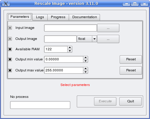
The resulting graphical application displays a window with several tabs:

Parameters is where you set the parameters and execute the application.
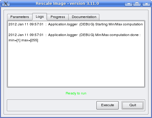
Logs is where you see the output given by the application during its execution.
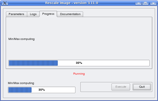
Progress is where you see a progress bar of the execution (not available for all applications).
Documentation is where you find a summary of the application documentation.

In this interface, every optional parameter has a check box that you have to tick if you want to set a value and use this parameter. The mandatory parameters cannot be unchecked.

The interface of the application is shown here as an example.

Python interface¶

The applications can also be accessed from Python, through a module named otbApplication. However, there are technical requirements to use it. If you use OTB through standalone packages, you should use the supplied environment script otbenv to properly setup variables such as PYTHONPATH and OTB_APPLICATION_PATH (on Unix systems, don’t forget to source the script). In other cases, you should set these variables depending on your configuration.

On Unix systems, it is typically available in the /usr/lib/otb/python directory. Depending on how you installed OTB, you may need to configure the environment variable PYTHONPATH to include this directory so that the module becomes available from Python.

On Windows, you can install the otb-python package, and the module will be available from an OSGeo4W shell automatically.

As for the command line and GUI launchers, the path to the application modules needs to be properly set with the OTB_APPLICATION_PATH environment variable. The standard location on Unix systems is /usr/lib/otb/applications. On Windows, the applications are available in the otb-bin OSGeo4W package, and the environment is configured automatically so you don’t need to tweak OTB_APPLICATION_PATH.

In the otbApplication module, two main classes can be manipulated :

Registry, which provides access to the list of available applications, and can create applications.
Application, the base class for all applications. This allows to interact with an application instance created by the Registry.

Here is one example of how to use Python to run the Smoothing application, changing the algorithm at each iteration.

#  Example on the use of the Smoothing application
#

# We will use sys.argv to retrieve arguments from the command line.
# Here, the script will accept an image file as first argument,
# and the basename of the output files, without extension.
from sys import argv

# The python module providing access to OTB applications is otbApplication
import otbApplication

# otbApplication.Registry can tell you what application are available
print "Available applications: "
print str( otbApplication.Registry.GetAvailableApplications() )

# Let's create the application with codename "Smoothing"
app = otbApplication.Registry.CreateApplication("Smoothing")

# We print the keys of all its parameter
print app.GetParametersKeys()

# First, we set the input image filename
app.SetParameterString("in", argv[1])

# The smoothing algorithm can be set with the "type" parameter key
# and can take 3 values: 'mean', 'gaussian', 'anidif'
for type in ['mean', 'gaussian', 'anidif']:

  print 'Running with ' + type + ' smoothing type'

  # Here we configure the smoothing algorithm
  app.SetParameterString("type", type)

  # Set the output filename, using the algorithm to differentiate the outputs
  app.SetParameterString("out", argv[2] + type + ".tif")

  # This will execute the application and save the output file
  app.ExecuteAndWriteOutput()

Numpy array processing¶

Input and output images to any OTB application in the form of numpy array is now possible in OTB python wrapping. The python wrapping only exposes OTB ApplicationEngine module which allow to access existing C++ applications. Due to blissful nature of ApplicationEngine’s loading mechanism no specific wrapping is required for each application.

Numpy extension to Python wrapping allows data exchange to application as an array rather than a disk file. Ofcourse, it is possible to load an image from file and then convert to numpy array or just provide a file as earlier via Application.SetParameterString(...).

This bridge that completes numpy and OTB makes it easy to plug OTB into any image processing chain via python code that uses GIS/Image processing tools such as GDAL, GRASS GIS, OSSIM that can deal with numpy.

Below code reads an input image using python pillow (PIL) and convert it to numpy array. This numpy array is used an input to the application via SetImageFromNumpyArray(...) method. The application used in this example is ExtractROI. After extracting a small area the output image is taken as numpy array with GetImageFromNumpyArray(...) method thus avoid wiriting output to a temporary file.

import sys
import os
import numpy as np
import otbApplication
from PIL import Image as PILImage

pilimage = PILImage.open('poupees.jpg')
npimage = np.asarray(pilimage)
inshow(pilimage)

ExtractROI = otbApplication.Registry.CreateApplication('ExtractROI')
ExtractROI.SetImageFromNumpyArray('in', npimage)
ExtractROI.SetParameterInt('startx', 140)
ExtractROI.SetParameterInt('starty', 120)
ExtractROI.SetParameterInt('sizex', 150)
ExtractROI.SetParameterInt('sizey', 150)
ExtractROI.Execute()

ExtractOutput = ExtractROI.GetImageAsNumpyArray('out')
output_pil_image = PILImage.fromarray(np.uint8(ExtractOutput))
imshow(output_pil_image)

In-memory connection¶

Applications are often use as parts of larger processing chains. Chaining applications currently requires to write/read back images between applications, resulting in heavy I/O operations and a significant amount of time dedicated to writing temporary files.

Since OTB 5.8, it is possible to connect an output image parameter from one application to the input image parameter of the next parameter. This results in the wiring of the internal ITK/OTB pipelines together, allowing to perform image streaming between the applications. There is therefore no more writing of temporary images. The last application of the processing chain is responsible for writing the final result images.

In-memory connection between applications is available both at the C++ API level and using the python bindings to the application presented in the Python interface section.

Here is a Python code sample connecting several applications together:

import otbApplication as otb

app1 = otb.Registry.CreateApplication("Smoothing")
app2 = otb.Registry.CreateApplication("Smoothing")
app3 = otb.Registry.CreateApplication("Smoothing")
app4 = otb.Registry.CreateApplication("ConcatenateImages")

app1.IN = argv[1]
app1.Execute()

# Connection between app1.out and app2.in
app2.SetParameterInputImage("in",app1.GetParameterOutputImage("out"))

# Execute call is mandatory to wire the pipeline and expose the
# application output. It does not write image
app2.Execute()

app3.IN = argv[1]

# Execute call is mandatory to wire the pipeline and expose the
# application output. It does not write image
app3.Execute()

# Connection between app2.out, app3.out and app4.il using images list
app4.AddImageToParameterInputImageList("il",app2.GetParameterOutputImage("out"));
app4.AddImageToParameterInputImageList("il",app3.GetParameterOutputImage("out"));

app4.OUT = argv[2]

# Call to ExecuteAndWriteOutput() both wires the pipeline and
# actually writes the output, only necessary for last application of
# the chain.
app4.ExecuteAndWriteOutput()

Note: Streaming will only work properly if the application internal implementation does not break it, for instance by using an internal writer to write intermediate data. In this case, execution should still be correct, but some intermediate data will be read or written.

QGIS interface¶

The processing toolbox¶

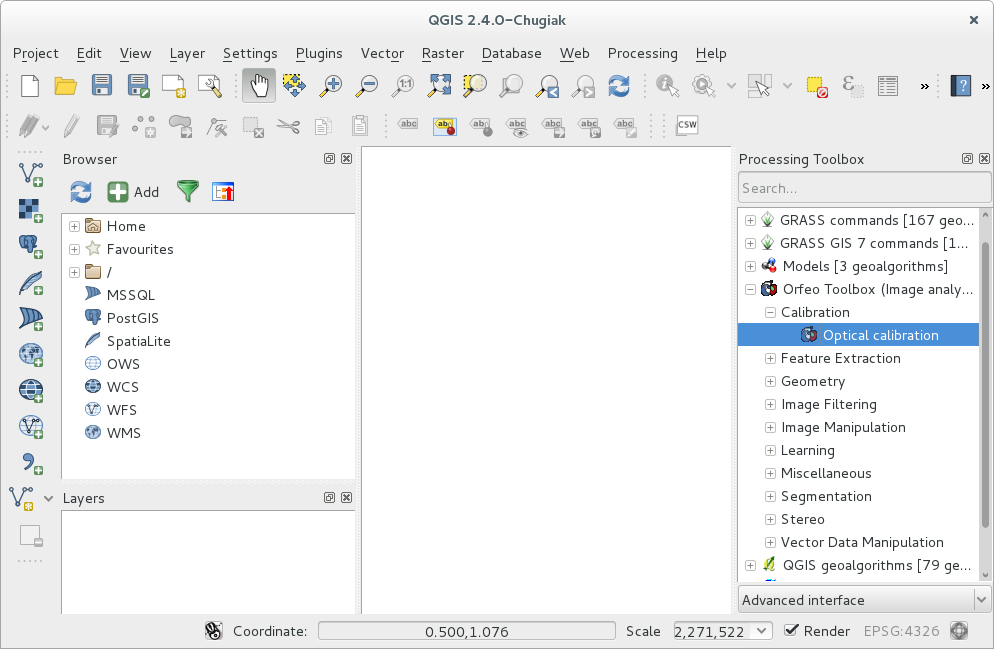
OTB applications are available from QGIS. Use them from the processing toolbox, which is accessible with Processing $\rightarrow$ ToolBox. Switch to “advanced interface” in the bottom of the application widget and OTB applications will be there.

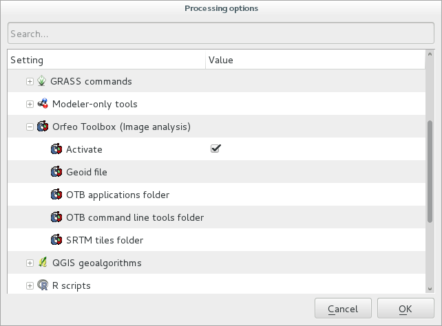
Using a custom OTB¶

If QGIS cannot find OTB, the “applications folder” and “binaries folder” can be set from the settings in the Processing $\rightarrow$ Settings $\rightarrow$ “service provider”.

On some versions of QGIS, if an existing OTB installation is found, the textfield settings will not be shown. To use a custom OTB instead of the existing one, you will need to replace the otbcli, otbgui and library files in QGIS installation directly.

Load and save parameters to XML¶

Since OTB 3.20, OTB applications parameters can be export/import to/from an XML file using inxml/outxml parameters. Those parameters are available in all applications.

An example is worth a thousand words

otbcli_BandMath -il input_image_1 input_image_2
                -exp "abs(im1b1 - im2b1)"
                -out output_image
                -outxml saved_applications_parameters.xml

Then, you can run the applications with the same parameters using the output XML file previously saved. For this, you have to use the inxml parameter:

otbcli_BandMath -inxml saved_applications_parameters.xml

Note that you can also overload parameters from command line at the same time

otbcli_BandMath -inxml saved_applications_parameters.xml
                -exp "(im1b1 - im2b1)"

In this case it will use as mathematical expression “(im1b1 - im2b1)” instead of “abs(im1b1 - im2b1)”.

Finally, you can also launch applications directly from the command-line launcher executable using the inxml parameter without having to declare the application name. Use in this case:

otbApplicationLauncherCommandLine -inxml saved_applications_parameters.xml

It will retrieve the application name and related parameters from the input XML file and launch in this case the BandMath applications.

Parallel execution with MPI¶

Provided that Orfeo ToolBox has been built with MPI and SPTW modules activated, it is possible to use MPI for massive parallel computation and writing of an output image. A simple call to mpirun before the command-line activates this behaviour, with the following logic. MPI writing is only triggered if:

OTB is built with MPI and SPTW,
The number of MPI processes is greater than 1,
The output filename is .tif or .vrt

In this case, the output image will be divided into several tiles according to the number of MPI processes specified to the mpirun command, and all tiles will be computed in parallel.

If the output filename extension is .tif, tiles will be written in parallel to a single Tiff file using SPTW (Simple Parallel Tiff Writer).

If the output filename extension is .vrt, each tile will be written to a separate Tiff file, and a global VRT file will be written.

Here is an example of MPI call on a cluster:

$ mpirun -np $nb_procs --hostfile $PBS_NODEFILE  \
  otbcli_BundleToPerfectSensor \
  -inp $ROOT/IMG_PHR1A_P_001/IMG_PHR1A_P_201605260427149_ORT_1792732101-001_R1C1.JP2 \
  -inxs $ROOT/IMG_PHR1A_MS_002/IMG_PHR1A_MS_201605260427149_ORT_1792732101-002_R1C1.JP2 \
  -out $ROOT/pxs.tif uint16 -ram 1024

  ------------ JOB INFO 1043196.tu-adm01 -------------

  JOBID           : 1043196.tu-adm01
  USER            : michelj
  GROUP           : ctsiap
  JOB NAME        : OTB_mpi
  SESSION         : 631249
  RES REQSTED     : mem=1575000mb,ncpus=560,place=free,walltime=04:00:00
  RES USED        : cpupercent=1553,cput=00:56:12,mem=4784872kb,ncpus=560,vmem=18558416kb,
  walltime=00:04:35
  BILLING         : 42:46:40 (ncpus x walltime)
  QUEUE           : t72h
  ACCOUNT         : null
  JOB EXIT CODE   : 0

------------ END JOB INFO 1043196.tu-adm01 ---------

One can see that the registration and pan-sharpening of the panchromatic and multi-spectral bands of a Pleiades image has been split among 560 cpus and took only 56 seconds.

Note that this MPI parallel invocation of applications is only available for command-line calls to OTB applications, and only for images output parameters.

Extended filenames¶

There are multiple ways to define geo-referencing information. For instance, one can use a geographic transform, a cartographic projection, or a sensor model with RPC coefficients. A single image may contain several of these elements, such as in the “ortho-ready” products: this is a type of product still in sensor geometry (the sensor model is supplied with the image) but it also contains an approximative geographic transform that can be used to have a quick estimate of the image localisation. For instance, your product may contain a “.TIF” file for the image, along with a “.RPB” file that contains the sensor model coefficients and an “.IMD” file that contains a cartographic projection.

This case leads to the following question: which geo-referencing element should be used when opening this image in OTB. In fact, it depends on the users need. For an orthorectification application, the sensor model must be used. In order to specify which information should be skipped, a syntax of extended filenames has been developed for both reading and writing.

The reader and writer extended file name support is based on the same syntax, only the options are different. To benefit from the extended file name mechanism, the following syntax is to be used:

Path/Image.ext?&key1=<value1>&key2=<value2>

Note that you’ll probably need to “quote” the filename, especially if calling applications from the bash command line.

Reader options¶

&geom=<path/filename.geom>

Contains the file name of a valid geom file
Use the content of the specified geom file instead of image-embedded geometric information
empty by default, use the image-embedded information if available

&sdataidx=<(int)idx>

Select the sub-dataset to read
0 by default

&resol=<(int)resolution factor>

Select the JPEG2000 sub-resolution image to read
0 by default

&bands=r1,r2,...,rn

Select a subset of bands from the input image
The syntax is inspired by Python indexing syntax with bands=r1,r2,r3,...,rn where each ri is a band range that can be :
- a single index (1-based) :
  - 2 means 2nd band
  - -1 means last band
- or a range of bands :
  - 3: means 3rd band until the last one
  - :-2 means the first bands until the second to last
  - 2:4 means bands 2,3 and 4
empty by default (all bands are read from the input image)

&skipcarto=<(bool)true>

Skip the cartographic information
Clears the projectionref, set the origin to $[0,0]$ and the spacing to $[1/max(1,r),1/max(1,r)]$ where $r$ is the resolution factor.
Keeps the keyword list
false by default

&skipgeom=<(bool)true>

Skip geometric information
Clears the keyword list
Keeps the projectionref and the origin/spacing information
false by default.

&skiprpctag=<(bool)true>

Skip the reading of internal RPC tags (see [sec:TypesofSensorModels] for details)
false by default.

Writer options¶

&writegeom=<(bool)false>

To activate writing of external geom file
true by default

&writerpctags=<(bool)true>

To activate writing of RPC tags in TIFF files
false by default

&gdal:co:<GDALKEY>=<VALUE>

To specify a gdal creation option
For gdal creation option information, see dedicated gdal documentation
None by default

&streaming:type=<VALUE>

Activates configuration of streaming through extended filenames
Override any previous configuration of streaming
Allows to configure the kind of streaming to perform
Available values are:
- auto: tiled or stripped streaming mode chosen automatically depending on TileHint read from input files
- tiled: tiled streaming mode
- stripped: stripped streaming mode
- none: explicitly deactivate streaming
Not set by default

&streaming:sizemode=<VALUE>

Allows to choose how the size of the streaming pieces is computed
Available values are:
- auto: size is estimated from the available memory setting by evaluating pipeline memory print
- height: size is set by setting height of strips or tiles
- nbsplits: size is computed from a given number of splits
Default is auto

&streaming:sizevalue=<VALUE>

Parameter for size of streaming pieces computation
Value is :
- if sizemode=auto: available memory in Mb
- if sizemode=height: height of the strip or tile in pixels
- if sizemode=nbsplits: number of requested splits for streaming
If not provided, the default value is set to 0 and result in different behaviour depending on sizemode (if set to height or nbsplits, streaming is deactivated, if set to auto, value is fetched from configuration or cmake configuration file)

&box=<startx>:<starty>:<sizex>:<sizey>

User defined parameters of output image region
The region must be set with 4 unsigned integers (the separator used is the colon ’:’). Values are:
- startx: first index on X (starting with 0)
- starty: first index on Y (starting with 0)
- sizex: size along X
- sizey: size along Y
The definition of the region follows the same convention as itk::Region definition in C++. A region is defined by two classes: the itk::Index and itk::Size classes. The origin of the region within the image with which it is associated is defined by Index

&bands=r1,r2,...,rn

Select a subset of bands from the output image
The syntax is inspired by Python indexing syntax with bands=r1,r2,r3,...,rn where each ri is a band range that can be :
- a single index (1-based) :
  - 2 means 2nd band
  - -1 means last band
- or a range of bands :
  - 3: means 3rd band until the last one
  - :-2 means the first bands until the second to last
  - 2:4 means bands 2,3 and 4
Empty by default (all bands are write from the output image)

The available syntax for boolean options are:

ON, On, on, true, True, 1 are available for setting a ’true’ boolean value
OFF, Off, off, false, False, 0 are available for setting a ’false’ boolean value