Image classification consists in extracting added-value information from images. Such processing methods
classify pixels within images into geographical connected zones with similar properties, and identified by a
common class label. The classification can be either unsupervised or supervised.
Unsupervised classification does not require any additional information about the properties of the input
image to classify it. On the contrary, supervised methods need a preliminary learning to be computed over
training datasets having similar properties than the image to classify, in order to build a classification
model.
The OTB classification is implemented as a generic Machine Learning framework, supporting several
possible machine learning libraries as backends. The base class otb::MachineLearningModel defines
this framework. As of now libSVM (the machine learning library historically integrated in
OTB), machine learning methods of OpenCV library ([14]) and also Shark machine learning
library ([67]) are available. Both supervised and unsupervised classifiers are supported in the
framework.
The current list of classifiers available through the same generic interface within the OTB is:
- LibSVM: Support Vector Machines classifier based on libSVM.
- SVM: Support Vector Machines classifier based on OpenCV, itself based on libSVM.
- Bayes: Normal Bayes classifier based on OpenCV.
- Boost: Boost classifier based on OpenCV.
- DT: Decision Tree classifier based on OpenCV.
- RF: Random Forests classifier based on the Random Trees in OpenCV.
- GBT: Gradient Boosted Tree classifier based on OpenCV (removed in version 3).
- KNN: K-Nearest Neighbors classifier based on OpenCV.
- ANN: Artificial Neural Network classifier based on OpenCV.
- SharkRF : Random Forests classifier based on Shark.
- SharkKM : KMeans unsupervised classifier based on Shark.
These models have a common interface, with the following major functions:
- SetInputListSample(InputListSampleType ⋆in) : set the list of input samples
- SetTargetListSample(TargetListSampleType ⋆in) : set the list of target samples
- Train() : train the model based on input samples
- Save(...) : saves the model to file
- Load(...) : load a model from file
- Predict(...) : predict a target value for an input sample
- PredictBatch(...) : prediction on a list of input samples
The PredictBatch(...) function can be multi-threaded when called either from a multi-threaded filter, or
from a single location. In the later case, it creates several threads using OpenMP. There is a factory
mechanism on top of the model class (see otb::MachineLearningModelFactory ). Given an input file,
the static function CreateMachineLearningModel(...) is able to instantiate a model of the right
type.
For unsupervised models, the target samples still have to be set. They won’t be used so you can fill a
ListSample with zeros.
The models are trained from a list of input samples, stored in a itk::Statistics::ListSample
. For supervised classifiers, they also need a list of targets associated to each input sample.
Whatever the source of samples, it has to be converted into a ListSample before being fed into the
model.
Then, model-specific parameters can be set. And finally, the Train() method starts the learning step. Once
the model is trained it can be saved to file using the function Save(). The following examples show how to
do that.
The source code for this example can be found in the file
Examples/Learning/TrainMachineLearningModelFromSamplesExample.cxx.
This example illustrates the use of the otb::SVMMachineLearningModel class, which inherits from the
otb::MachineLearningModel class. This class allows the estimation of a classification model (supervised
learning) from samples. In this example, we will train an SVM model with 4 output classes, from 1000
randomly generated training samples, each of them having 7 components. We start by including the
appropriate header files.
// List sample generator #include "otbListSampleGenerator.h" // Random number generator
// SVM model Estimator #include "otbSVMMachineLearningModel.h"
The input parameters of the sample generator and of the SVM classifier are initialized.
int nbSamples = 1000; int nbSampleComponents = 7; int nbClasses = 4;
Two lists are generated into a itk::Statistics::ListSample which is the structure used
to handle both lists of samples and of labels for the machine learning classes derived from
otb::MachineLearningModel . The first list is composed of feature vectors representing multi-component
samples, and the second one is filled with their corresponding class labels. The list of labels is composed of
scalar values.
// Input related typedefs typedef float InputValueType;
typedef itk::VariableLengthVector<InputValueType> InputSampleType;
typedef itk::Statistics::ListSample<InputSampleType> InputListSampleType; // Target related typedefs
typedef int TargetValueType; typedef itk::FixedArray<TargetValueType, 1> TargetSampleType;
typedef itk::Statistics::ListSample<TargetSampleType> TargetListSampleType;
InputListSampleType::Pointer InputListSample = InputListSampleType::New();
TargetListSampleType::Pointer TargetListSample = TargetListSampleType::New();
InputListSample->SetMeasurementVectorSize(nbSampleComponents);
In this example, the list of multi-component training samples is randomly filled with a random number
generator based on the itk::Statistics::MersenneTwisterRandomVariateGenerator class. Each
component’s value is generated from a normal law centered around the corresponding class label of each
sample multiplied by 100, with a standard deviation of 10.
itk::Statistics::MersenneTwisterRandomVariateGenerator::Pointer randGen;
randGen = itk::Statistics::MersenneTwisterRandomVariateGenerator::GetInstance();
// Filling the two input training lists for (int i = 0; i < nbSamples; ++i)
{ InputSampleType sample; TargetValueType label = (i % nbClasses) + 1;
// Multi-component sample randomly filled from a normal law for each component
sample.SetSize(nbSampleComponents); for (int itComp = 0; itComp < nbSampleComponents; ++itComp)
{ sample[itComp] = randGen->GetNormalVariate(100 ⋆ label, 10); }
InputListSample->PushBack(sample); TargetListSample->PushBack(label); }
Once both sample and label lists are generated, the second step consists in declaring the machine learning
classifier. In our case we use an SVM model with the help of the otb::SVMMachineLearningModel class
which is derived from the otb::MachineLearningModel class. This pure virtual class is based on the
machine learning framework of the OpenCV library ([14]) which handles other classifiers than the SVM.
typedef otb::SVMMachineLearningModel<InputValueType, TargetValueType> SVMType;
SVMType::Pointer SVMClassifier = SVMType::New(); SVMClassifier->SetInputListSample(InputListSample);
SVMClassifier->SetTargetListSample(TargetListSample); SVMClassifier->SetKernelType(CvSVM::LINEAR);
Once the classifier is parametrized with both input lists and default parameters, except for the kernel type in
our example of SVM model estimation, the model training is computed with the Train method. Finally, the
Save method exports the model to a text file. All the available classifiers based on OpenCV are
implemented with these interfaces. Like for the SVM model training, the other classifiers can be
parametrized with specific settings.
SVMClassifier->Train(); SVMClassifier->Save(outputModelFileName);
The source code for this example can be found in the file
Examples/Learning/TrainMachineLearningModelFromImagesExample.cxx.
This example illustrates the use of the otb::MachineLearningModel class. This class allows the
estimation of a classification model (supervised learning) from images. In this example, we will train an
SVM with 4 classes. We start by including the appropriate header files.
// List sample generator #include "otbListSampleGenerator.h"
// Extract a ROI of the vectordata #include "otbVectorDataIntoImageProjectionFilter.h"
// SVM model Estimator #include "otbSVMMachineLearningModel.h"
In this framework, we must transform the input samples store in a vector data into a
itk::Statistics::ListSample which is the structure compatible with the machine learning classes. On
the one hand, we are using feature vectors for the characterization of the classes, and on the other hand, the
class labels are scalar values. We first re-project the input vector data over the input image, using the
otb::VectorDataIntoImageProjectionFilter class. To convert the input samples store in a vector
data into a itk::Statistics::ListSample , we use the otb::ListSampleGenerator
class.
// VectorData projection filter typedef otb::VectorDataIntoImageProjectionFilter<VectorDataType, InputImageType>
VectorDataReprojectionType;
InputReaderType::Pointer inputReader = InputReaderType::New(); inputReader->SetFileName(inputImageFileName);
InputImageType::Pointer image = inputReader->GetOutput(); image->UpdateOutputInformation();
// Read the Vectordata VectorDataReaderType::Pointer vectorReader = VectorDataReaderType::New();
vectorReader->SetFileName(trainingShpFileName); vectorReader->Update();
VectorDataType::Pointer vectorData = vectorReader->GetOutput(); vectorData->Update();
VectorDataReprojectionType::Pointer vdreproj = VectorDataReprojectionType::New();
vdreproj->SetInputImage(image); vdreproj->SetInput(vectorData);
vdreproj->SetUseOutputSpacingAndOriginFromImage(false); vdreproj->Update();
typedef otb::ListSampleGenerator<InputImageType, VectorDataType>
ListSampleGeneratorType;
ListSampleGeneratorType::Pointer sampleGenerator; sampleGenerator = ListSampleGeneratorType::New();
sampleGenerator->SetInput(image); sampleGenerator->SetInputVectorData(vdreproj->GetOutput());
sampleGenerator->SetClassKey("Class"); sampleGenerator->Update();
Now, we need to declare the machine learning model which will be used by the classifier. In this example,
we train an SVM model. The otb::SVMMachineLearningModel class inherits from the pure virtual class
otb::MachineLearningModel which is templated over the type of values used for the measures and the
type of pixels used for the labels. Most of the classification and regression algorithms available through this
interface in OTB is based on the OpenCV library [14]. Specific methods can be used to set classifier
parameters. In the case of SVM, we set here the type of the kernel. Other parameters are let with their
default values.
typedef otb::SVMMachineLearningModel <InputImageType::InternalPixelType,
ListSampleGeneratorType::ClassLabelType> SVMType;
SVMType::Pointer SVMClassifier = SVMType::New();
SVMClassifier->SetInputListSample(sampleGenerator->GetTrainingListSample());
SVMClassifier->SetTargetListSample(sampleGenerator->GetTrainingListLabel());
SVMClassifier->SetKernelType(CvSVM::LINEAR);
The machine learning interface is generic and gives access to other classifiers. We now train the SVM
model using the Train and save the model to a text file using the Save method.
SVMClassifier->Train(); SVMClassifier->Save(outputModelFileName);
You can now use the Predict method which takes a itk::Statistics::ListSample as input and
estimates the label of each input sample using the model. Finally, the otb::ImageClassificationModel
inherits from the itk::ImageToImageFilter and allows classifying pixels in the input image by
predicting their labels using a model.
For the prediction step, the usual process is to:
- Load an existing model from a file.
- Convert the data to predict into a ListSample.
- Run the PredictBatch(...) function.
There is an image filter that perform this step on a whole image, supporting streaming and multi-threading:
otb::ImageClassificationFilter .
The source code for this example can be found in the file
Examples/Classification/SupervisedImageClassificationExample.cxx.
In OTB, a generic streamed filter called otb::ImageClassificationFilter is available to classify any
input multi-channel image according to an input classification model file. This filter is generic because it
works with any classification model type (SVM, KNN, Artificial Neural Network,...) generated within the
OTB generic Machine Learning framework based on OpenCV ([14]). The input model file is smartly parsed
according to its content in order to identify which learning method was used to generate it. Once the
classification method and model are known, the input image can be classified. More details are
given in subsections ?? and ?? to generate a classification model either from samples or from
images. In this example we will illustrate its use. We start by including the appropriate header
files.
#include "otbMachineLearningModelFactory.h" #include "otbImageClassificationFilter.h"
We will assume double precision input images and will also define the type for the labeled
pixels.
const unsigned int Dimension = 2; typedef double PixelType;
typedef unsigned short LabeledPixelType;
Our classifier is generic enough to be able to process images with any number of bands. We read the input
image as a otb::VectorImage . The labeled image will be a scalar image.
typedef otb::VectorImage<PixelType, Dimension> ImageType;
typedef otb::Image<LabeledPixelType, Dimension> LabeledImageType;
We can now define the type for the classifier filter, which is templated over its input and output image
types.
typedef otb::ImageClassificationFilter<ImageType, LabeledImageType>
ClassificationFilterType;
typedef ClassificationFilterType::ModelType ModelType;
Moreover, it is necessary to define a otb::MachineLearningModelFactory which is templated over its
input and output pixel types. This factory is used to parse the input model file and to define which
classification method to use.
typedef otb::MachineLearningModelFactory<PixelType, LabeledPixelType>
MachineLearningModelFactoryType;
And finally, we define the reader and the writer. Since the images to classify can be very big, we will use a
streamed writer which will trigger the streaming ability of the classifier.
typedef otb::ImageFileReader<ImageType> ReaderType;
typedef otb::ImageFileWriter<LabeledImageType> WriterType;
We instantiate the classifier and the reader objects and we set the existing model obtained in a previous
training step.
ClassificationFilterType::Pointer filter = ClassificationFilterType::New();
ReaderType::Pointer reader = ReaderType::New(); reader->SetFileName(infname);
The input model file is parsed according to its content and the generated model is then loaded within the
otb::ImageClassificationFilter .
ModelType::Pointer model; model = MachineLearningModelFactoryType::CreateMachineLearningModel(
modelfname,
MachineLearningModelFactoryType::ReadMode);
model->Load(modelfname); filter->SetModel(model);
We plug the pipeline and trigger its execution by updating the output of the writer.
filter->SetInput(reader->GetOutput()); WriterType::Pointer writer = WriterType::New();
writer->SetInput(filter->GetOutput()); writer->SetFileName(outfname); writer->Update();
The classifiers are integrated in several OTB Applications. There is a base class that provides an easy access
to all the classifiers: otb::Wrapper::LearningApplicationBase . As each machine learning model has
a specific set of parameters, the base class LearningApplicationBase knows how to expose each type of
classifier with its dedicated parameters (a task that is a bit tedious so we want to implement it only once).
The DoInit() method creates a choice parameter named classifier which contains the different
supported classifiers along with their parameters.
The function Train(...) provide an easy way to train the selected classifier, with the corresponding
parameters, and save the model to file.
On the other hand, the function Classify(...) allows to load a model from file and apply it on a list of
samples.
Kernel based learning methods in general and the Support Vector Machines (SVM) in particular, have been
introduced in the last years in learning theory for classification and regression tasks, [132]. SVM have
been successfully applied to text categorization, [74], and face recognition, [102]. Recently,
they have been successfully used for the classification of hyperspectral remote-sensing images,
[15].
Simply stated, the approach consists in searching for the separating surface between 2 classes by the
determination of the subset of training samples which best describes the boundary between the 2 classes.
These samples are called support vectors and completely define the classification system. In the case where
the two classes are nonlinearly separable, the method uses a kernel expansion in order to make projections
of the feature space onto higher dimensionality spaces where the separation of the classes becomes
linear.
This subsection reminds the basic principles of SVM learning and classification. A good tutorial on SVM
can be found in, [17].
We have N samples represented by the couple (yi,xi),i = 1…N where yi ∈{-1,+1} is the class label and
xi ∈ℝn is the feature vector of dimension n. A classifier is a function
 where
α are the classifier parameters. The SVM finds the optimal separating hyperplane which fulfills the
following constraints :
where
α are the classifier parameters. The SVM finds the optimal separating hyperplane which fulfills the
following constraints :
- The samples with labels +1 and -1 are on different sides of the hyperplane.
- The distance of the closest vectors to the hyperplane is maximised. These are the support
vectors (SV) and this distance is called the margin.
The separating hyperplane has the equation
 with
w being its normal vector and x being any point of the hyperplane. The orthogonal distance to
the origin is given by
with
w being its normal vector and x being any point of the hyperplane. The orthogonal distance to
the origin is given by  . Vectors located outside the hyperplane have either w ⋅x +b > 0 or
w ⋅x +b < 0.
. Vectors located outside the hyperplane have either w ⋅x +b > 0 or
w ⋅x +b < 0.
Therefore, the classifier function can be written as

The SVs are placed on two hyperplanes which are parallel to the optimal separating one. In order to find the
optimal hyperplane, one sets w and b :

Since there must not be any vector inside the margin, the following constraint can be used:

 which can be rewritten as
The orthogonal distances of the 2 parallel hyperplanes to the origin are  and
and  . Therefore the
modulus of the margin is equal to
. Therefore the
modulus of the margin is equal to  and it has to be maximised.
Thus, the problem to be solved is:
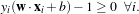
- Find w and b which minimise

- under the constraint : yi(w ⋅xi+b) ≥ 1 i = 1…N.
This problem can be solved by using the Lagrange multipliers with one multiplier per sample. It can be
shown that only the support vectors will have a positive Lagrange multiplier.
In the case where the two classes are not exactly linearly separable, one can modify the constraints above by
using


If ξi > 1, one considers that the sample is wrong. The function which has then to be minimised is
 ∥w∥2 +C
 ;, where C is a tolerance parameter. The optimisation problem is the same than in the
linear case, but one multiplier has to be added for each new constraint ξi ≥ 0.
;, where C is a tolerance parameter. The optimisation problem is the same than in the
linear case, but one multiplier has to be added for each new constraint ξi ≥ 0.
If the decision surface needs to be non-linear, this solution cannot be applied and the kernel approach has to
be adopted.
One drawback of the SVM is that, in their basic version, they can only solve two-class problems. Some
works exist in the field of multi-class SVM (see [4, 136], and the comparison made by [59]), but they are
not used in our system.
You have to be aware that to achieve better convergence of the algorithm it is strongly advised to normalize
feature vector components in the [-1;1] interval.
For problems with N > 2 classes, one can choose either to train N SVM (one class against all the others), or
to train N ×(N -1) SVM (one class against each of the others). In the second approach, which is the one
that we use, the final decision is taken by choosing the class which is most often selected by the whole set of
SVM.
The Random Forests algorithm is also available in OTB machine learning framework. This model builds a
set of decision trees. Each tree may not give a reliable prediction, but taking them together, they form
a robust classifier. The prediction of this model is the mode of the predictions of individual
trees.
There are two implementations: one in OpenCV and the other on in Shark. The Shark implementation has a
noteworthy advantage: the training step is parallel. It uses the following parameters:
- The number of trees to train
- The number of random attributes to investigate at each node
- The maximum node size to decide a split
- The ratio of the original training dataset to use as the out of bag sample
Except these specific parameter, its usage is exactly the same as the other machine learning models (such as
the SVM model).
OTB has developed a specific interface for user-defined kernels. However, the following functions use a
deprecated OTB interface. The code source for these Generic Kernels has been removed from the official
repository. It is now available as a remote module: GKSVM.
A function k(⋅,⋅) is considered to be a kernel when:
∀g(⋅) ∈ 2(Rn) 2(Rn) | so that ∫
g(x)2dx be finite, | (19.1)
|
| then ∫
k(x,y)g(x)g(y)dxdy ≥ 0, | | |
which is known as the Mercer condition.
When defined through the OTB, a kernel is a class that inherits from GenericKernelFunctorBase. Several
virtual functions have to be overloaded:
- The Evaluate function, which implements the behavior of the kernel itself. For instance, the
classical linear kernel could be re-implemented with:
double
MyOwnNewKernel
::Evaluate ( const svm_node ⋆ x, const svm_node ⋆ y,
const svm_parameter & param ) const
{
return this->dot(x,y);
}
This simple example shows that the classical dot product is already implemented into
otb::GenericKernelFunctorBase::dot() as a protected function.
- The Update() function which synchronizes local variables and their integration into the initial SVM
procedure. The following examples will show the way to use it.
Some pre-defined generic kernels have already been implemented in OTB:
- otb::MixturePolyRBFKernelFunctor which implements a linear mixture of a polynomial
and a RBF kernel;
- otb::NonGaussianRBFKernelFunctor which implements a non gaussian RBF kernel;
- otb::SpectralAngleKernelFunctor, a kernel that integrates the Spectral Angle, instead of
the Euclidean distance, into an inverse multiquadric kernel. This kernel may be appropriated
when using multispectral data.
- otb::ChangeProfileKernelFunctor, a kernel which is dedicated to the supervized
classification of the multiscale change profile presented in section 21.5.1.
The source code for this example can be found in the file
Examples/Learning/SVMGenericKernelImageModelEstimatorExample.cxx.
This example illustrates the modifications to be added to the use of otb::SVMImageModelEstimator in
order to add a user defined kernel. This initial program has been explained in section ??.
The first thing to do is to include the header file for the new kernel.
#include "otbSVMImageModelEstimator.h" #include "otbMixturePolyRBFKernelFunctor.h"
Once the otb::SVMImageModelEstimator is instantiated, it is possible to add the new kernel and its
parameters.
Then in addition to the initial code:
EstimatorType::Pointer svmEstimator = EstimatorType::New();
svmEstimator->SetSVMType(C_SVC); svmEstimator->SetInputImage(inputReader->GetOutput());
svmEstimator->SetTrainingImage(trainingReader->GetOutput());
The instantiation of the kernel is to be implemented. The kernel which is used here is a linear combination
of a polynomial kernel and an RBF one. It is written as
 with
k1(x,y) =
with
k1(x,y) =  d and k2(x,y) = exp
 . Then, the specific parameters of this kernel
are:
. Then, the specific parameters of this kernel
are:
- Mixture (μ),
- GammaPoly (γ1),
- CoefPoly (c0),
- DegreePoly (d),
- GammaRBF (γ2).
Their instantiations are achieved through the use of the SetValue function.
otb::MixturePolyRBFKernelFunctor myKernel; myKernel.SetValue("Mixture", 0.5);
myKernel.SetValue("GammaPoly", 1.0); myKernel.SetValue("CoefPoly", 0.0);
myKernel.SetValue("DegreePoly", 1); myKernel.SetValue("GammaRBF", 1.5); myKernel.Update();
Once the kernel’s parameters are affected and the kernel updated, the connection to
otb::SVMImageModelEstimator takes place here.
svmEstimator->SetKernelFunctor(&myKernel); svmEstimator->SetKernelType(GENERIC);
The model estimation procedure is triggered by calling the estimator’s Update method.
The rest of the code remains unchanged...
svmEstimator->SaveModel(outputModelFileName);
In the file outputModelFileName a specific line will appear when using a generic kernel. It gives the name
of the kernel and its parameters name and value.
The source code for this example can be found in the file
Examples/Learning/SVMGenericKernelImageClassificationExample.cxx.
This example illustrates the modifications to be added to use the otb::SVMClassifier class for
performing SVM classification on images with a user-defined kernel. In this example, we will use an SVM
model estimated in the previous section to separate between water and non-water pixels by using the RGB
values only. The first thing to do is include the header file for the class as well as the header of the
appropriated kernel to be used.
#include "otbSVMClassifier.h" #include "otbMixturePolyRBFKernelFunctor.h"
We need to declare the SVM model which is to be used by the classifier. The SVM model is templated over
the type of value used for the measures and the type of pixel used for the labels.
typedef otb::SVMModel<PixelType, LabelPixelType> ModelType; ModelType::Pointer model = ModelType::New();
After instantiation, we can load a model saved to a file (see section ?? for an example of model estimation
and storage to a file).
When using a user defined kernel, an explicit instantiation has to be performed.
otb::MixturePolyRBFKernelFunctor myKernel; model->SetKernelFunctor(&myKernel);
Then, the rest of the classification program remains unchanged.
model->LoadModel(modelFilename);
The KMeans algorithm has been implemented in Shark library, and has been wrapped in the OTB machine
learning framework. It is the first unsupervised algorithm in this framework. It can be used in the same way
as other machine learning models. Remember that even if unsupervised model don’t use a label information
on the samples, the target ListSample still has to be set in MachineLearningModel. A ListSample filled
with zeros can be used.
This model uses a hard clustering model with the following parameters:
- The maximum number of iterations
- The number of centroids (K)
- An option to normalize input samples
As with Shark Random Forests, the training step is parallel.
The source code for this example can be found in the file
Examples/Classification/ScalarImageKmeansClassifier.cxx.
This example shows how to use the KMeans model for classifying the pixel of a scalar image.
The itk::Statistics::ScalarImageKmeansImageFilter is used for taking a scalar image and
applying the K-Means algorithm in order to define classes that represents statistical distributions of
intensity values in the pixels. The classes are then used in this filter for generating a labeled image where
every pixel is assigned to one of the classes.
#include "otbImage.h" #include "otbImageFileReader.h" #include "otbImageFileWriter.h"
#include "itkScalarImageKmeansImageFilter.h"
First we define the pixel type and dimension of the image that we intend to classify. With this image type
we can also declare the otb::ImageFileReader needed for reading the input image, create one and set
its input filename.
typedef signed short PixelType; const unsigned int Dimension = 2;
typedef otb::Image<PixelType, Dimension> ImageType; typedef otb::ImageFileReader<ImageType> ReaderType;
ReaderType::Pointer reader = ReaderType::New(); reader->SetFileName(inputImageFileName);
With the ImageType we instantiate the type of the itk::ScalarImageKmeansImageFilter that will
compute the K-Means model and then classify the image pixels.
typedef itk::ScalarImageKmeansImageFilter<ImageType> KMeansFilterType;
KMeansFilterType::Pointer kmeansFilter = KMeansFilterType::New();
kmeansFilter->SetInput(reader->GetOutput()); const unsigned int numberOfInitialClasses = atoi(argv[4]);
In general the classification will produce as output an image whose pixel values are integers associated to
the labels of the classes. Since typically these integers will be generated in order (0, 1, 2, ...N), the output
image will tend to look very dark when displayed with naive viewers. It is therefore convenient
to have the option of spreading the label values over the dynamic range of the output image
pixel type. When this is done, the dynamic range of the pixels is divided by the number of
classes in order to define the increment between labels. For example, an output image of 8
bits will have a dynamic range of [0:255], and when it is used for holding four classes, the
non-contiguous labels will be (0, 64, 128, 192). The selection of the mode to use is done with the method
SetUseContiguousLabels().
const unsigned int useNonContiguousLabels = atoi(argv[3]);
kmeansFilter->SetUseNonContiguousLabels(useNonContiguousLabels);
For each one of the classes we must provide a tentative initial value for the mean of the class. Given that this
is a scalar image, each one of the means is simply a scalar value. Note however that in a general case of
K-Means, the input image would be a vector image and therefore the means will be vectors of the same
dimension as the image pixels.
for (unsigned k = 0; k < numberOfInitialClasses; ++k) {
const double userProvidedInitialMean = atof(argv[k + argoffset]);
kmeansFilter->AddClassWithInitialMean(userProvidedInitialMean); }
The itk::ScalarImageKmeansImageFilter is predefined for producing an 8 bits scalar image as
output. This output image contains labels associated to each one of the classes in the K-Means
algorithm. In the following lines we use the OutputImageType in order to instantiate the type of a
otb::ImageFileWriter . Then create one, and connect it to the output of the classification
filter.
typedef KMeansFilterType::OutputImageType OutputImageType;
typedef otb::ImageFileWriter<OutputImageType> WriterType; WriterType::Pointer writer = WriterType::New();
writer->SetInput(kmeansFilter->GetOutput()); writer->SetFileName(outputImageFileName);
We are now ready for triggering the execution of the pipeline. This is done by simply invoking the
Update() method in the writer. This call will propagate the update request to the reader and then to the
classifier.
try { writer->Update(); } catch (itk::ExceptionObject& excp) {
std::cerr << "Problem encountered while writing "; std::cerr << " image file : " << argv[2] << std::endl;
std::cerr << excp << std::endl; return EXIT_FAILURE; }
At this point the classification is done, the labeled image is saved in a file, and we can take a look at
the means that were found as a result of the model estimation performed inside the classifier
filter.
KMeansFilterType::ParametersType estimatedMeans = kmeansFilter->GetFinalMeans();
const unsigned int numberOfClasses = estimatedMeans.Size();
for (unsigned int i = 0; i < numberOfClasses; ++i) { std::cout << "cluster[" << i << "] ";
std::cout << " estimated mean : " << estimatedMeans[i] << std::endl; }
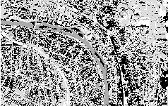
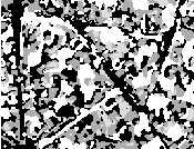
Figure 19.1 illustrates the effect of this filter with three classes. The means can be estimated by
ScalarImageKmeansModelEstimator.cxx.
The source code for this example can be found in the file
Examples/Classification/ScalarImageKmeansModelEstimator.cxx.
This example shows how to compute the KMeans model of an Scalar Image.
The itk::Statistics::KdTreeBasedKmeansEstimator is used for taking a scalar image and applying
the K-Means algorithm in order to define classes that represents statistical distributions of intensity values
in the pixels. One of the drawbacks of this technique is that the spatial distribution of the pixels is not
considered at all. It is common therefore to combine the classification resulting from K-Means with other
segmentation techniques that will use the classification as a prior and add spatial information to it in order
to produce a better segmentation.
// Create a List from the scalar image typedef itk::Statistics::ImageToListSampleAdaptor<ImageType> AdaptorType;
AdaptorType::Pointer adaptor = AdaptorType::New(); adaptor->SetImage(reader->GetOutput());
// Define the Measurement vector type from the AdaptorType // Create the K-d tree structure
typedef itk::Statistics::WeightedCentroidKdTreeGenerator< AdaptorType>
TreeGeneratorType; TreeGeneratorType::Pointer treeGenerator = TreeGeneratorType::New();
treeGenerator->SetSample(adaptor); treeGenerator->SetBucketSize(16); treeGenerator->Update();
typedef TreeGeneratorType::KdTreeType TreeType;
typedef itk::Statistics::KdTreeBasedKmeansEstimator<TreeType> EstimatorType;
EstimatorType::Pointer estimator = EstimatorType::New(); const unsigned int numberOfClasses = 4;
EstimatorType::ParametersType initialMeans(numberOfClasses); initialMeans[0] = 25.0;
initialMeans[1] = 125.0; initialMeans[2] = 250.0; estimator->SetParameters(initialMeans);
estimator->SetKdTree(treeGenerator->GetOutput()); estimator->SetMaximumIteration(200);
estimator->SetCentroidPositionChangesThreshold(0.0); estimator->StartOptimization();
EstimatorType::ParametersType estimatedMeans = estimator->GetParameters();
for (unsigned int i = 0; i < numberOfClasses; ++i) { std::cout << "cluster[" << i << "] " << std::endl;
std::cout << " estimated mean : " << estimatedMeans[i] << std::endl; }
The source code for this example can be found in the file
Examples/Classification/KMeansImageClassificationExample.cxx.
The K-Means classification proposed by ITK for images is limited to scalar images and is not streamed. In
this example, we show how the use of the otb::KMeansImageClassificationFilter allows for a
simple implementation of a K-Means classification application. We will start by including the appropirate
header file.
#include "otbKMeansImageClassificationFilter.h"
We will assume double precision input images and will also define the type for the labeled
pixels.
const unsigned int Dimension = 2; typedef double PixelType;
typedef unsigned short LabeledPixelType;
Our classifier will be generic enough to be able to process images with any number of bands. We read the
images as otb::VectorImage s. The labeled image will be a scalar image.
typedef otb::VectorImage<PixelType, Dimension> ImageType;
typedef otb::Image<LabeledPixelType, Dimension> LabeledImageType;
We can now define the type for the classifier filter, which is templated over its input and output image
types.
typedef otb::KMeansImageClassificationFilter<ImageType, LabeledImageType> ClassificationFilterType;
typedef ClassificationFilterType::KMeansParametersType KMeansParametersType;
And finally, we define the reader and the writer. Since the images to classify can be very big, we will use a
streamed writer which will trigger the streaming ability of the classifier.
typedef otb::ImageFileReader<ImageType> ReaderType;
typedef otb::ImageFileWriter<LabeledImageType> WriterType;
We instantiate the classifier and the reader objects and we set their parameters. Please note the call
of the GenerateOutputInformation() method on the reader in order to have available the
information about the input image (size, number of bands, etc.) without needing to actually read the
image.
ClassificationFilterType::Pointer filter = ClassificationFilterType::New();
ReaderType::Pointer reader = ReaderType::New(); reader->SetFileName(infname);
reader->GenerateOutputInformation();
The classifier needs as input the centroids of the classes. We declare the parameter vector, and we read the
centroids from the arguments of the program.
const unsigned int sampleSize = ClassificationFilterType::MaxSampleDimension;
const unsigned int parameterSize = nbClasses ⋆ sampleSize; KMeansParametersType parameters;
parameters.SetSize(parameterSize); parameters.Fill(0); for (unsigned int i = 0; i < nbClasses; ++i)
{ for (unsigned int j = 0; j < reader->GetOutput()->GetNumberOfComponentsPerPixel(); ++j)
{ parameters[i ⋆ sampleSize + j] = atof(argv[4 + i ⋆
reader->GetOutput()->GetNumberOfComponentsPerPixel() + j]);
} } std::cout << "Parameters: " << parameters << std::endl;
We set the parameters for the classifier, we plug the pipeline and trigger its execution by updating the output
of the writer.
filter->SetCentroids(parameters); filter->SetInput(reader->GetOutput());
WriterType::Pointer writer = WriterType::New(); writer->SetInput(filter->GetOutput());
writer->SetFileName(outfname); writer->Update();
The source code for this example can be found in the file
Examples/Classification/KdTreeBasedKMeansClustering.cxx.
K-means clustering is a popular clustering algorithm because it is simple and usually converges to a
reasonable solution. The k-means algorithm works as follows:
- Obtains the initial k means input from the user.
- Assigns each measurement vector in a sample container to its closest mean among the k
number of means (i.e., update the membership of each measurement vectors to the nearest of
the k clusters).
- Calculates each cluster’s mean from the newly assigned measurement vectors (updates the
centroid (mean) of k clusters).
- Repeats step 2 and step 3 until it meets the termination criteria.
The most common termination criteria is that if there is no measurement vector that changes its cluster
membership from the previous iteration, then the algorithm stops.
The itk::Statistics::KdTreeBasedKmeansEstimator is a variation of this logic. The k-means
clustering algorithm is computationally very expensive because it has to recalculate the mean at each
iteration. To update the mean values, we have to calculate the distance between k means and each and every
measurement vector. To reduce the computational burden, the KdTreeBasedKmeansEstimator uses a special
data structure: the k-d tree ( itk::Statistics::KdTree ) with additional information. The additional
information includes the number and the vector sum of measurement vectors under each node under the tree
architecture.
With such additional information and the k-d tree data structure, we can reduce the computational cost of
the distance calculation and means. Instead of calculating each measurement vectors and k means, we can
simply compare each node of the k-d tree and the k means. This idea of utilizing a k-d tree can be found in
multiple articles [5] [104] [78]. Our implementation of this scheme follows the article by the Kanungo et al
[78].
We use the itk::Statistics::ListSample as the input sample, the itk::Vector as the
measurement vector. The following code snippet includes their header files.
#include "itkVector.h" #include "itkListSample.h"
Since this k-means algorithm requires a itk::Statistics::KdTree object as an input, we include the
KdTree class header file. As mentioned above, we need a k-d tree with the vector sum and the number of
measurement vectors. Therefore we use the itk::Statistics::WeightedCentroidKdTreeGenerator
instead of the itk::Statistics::KdTreeGenerator that generate a k-d tree without such additional
information.
#include "itkKdTree.h" #include "itkWeightedCentroidKdTreeGenerator.h"
The KdTreeBasedKmeansEstimator class is the implementation of the k-means algorithm. It does not create
k clusters. Instead, it returns the mean estimates for the k clusters.
#include "itkKdTreeBasedKmeansEstimator.h"
To generate the clusters, we must create k instances of itk::Statistics::EuclideanDistanceMetric
function as the membership functions for each cluster and plug that—along with a sample—into an
itk::Statistics::SampleClassifierFilter object to get a itk::Statistics::MembershipSample
that stores pairs of measurement vectors and their associated class labels (k labels).
#include "itkMinimumDecisionRule.h" #include "itkSampleClassifierFilter.h"
We will fill the sample with random variables from two normal distribution using the
itk::Statistics::NormalVariateGenerator .
#include "itkNormalVariateGenerator.h"
Since the NormalVariateGenerator class only supports 1-D, we define our measurement
vector type as one component vector. We then, create a ListSample object for data inputs. Each
measurement vector is of length 1. We set this using the SetMeasurementVectorSize() method.
typedef itk::Vector<double, 1> MeasurementVectorType;
typedef itk::Statistics::ListSample<MeasurementVectorType> SampleType;
SampleType::Pointer sample = SampleType::New(); sample->SetMeasurementVectorSize(1);
The following code snippet creates a NormalVariateGenerator object. Since the random variable generator
returns values according to the standard normal distribution (The mean is zero, and the standard deviation is
one), before pushing random values into the sample, we change the mean and standard deviation.
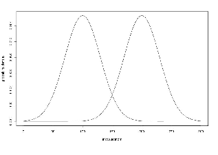
We want two normal (Gaussian) distribution data. We have two for loops. Each for loop uses
different mean and standard deviation. Before we fill the sample with the second distribution data,
we call Initialize(random seed) method, to recreate the pool of random variables in the
normalGenerator.
To see the probability density plots from the two distribution, refer to the Figure 19.2.
typedef itk::Statistics::NormalVariateGenerator NormalGeneratorType;
NormalGeneratorType::Pointer normalGenerator = NormalGeneratorType::New();
normalGenerator->Initialize(101); MeasurementVectorType mv; double mean = 100;
double standardDeviation = 30; for (unsigned int i = 0; i < 100; ++i)
{ mv[0] = (normalGenerator->GetVariate() ⋆ standardDeviation) + mean;
sample->PushBack(mv); } normalGenerator->Initialize(3024); mean = 200;
standardDeviation = 30; for (unsigned int i = 0; i < 100; ++i) {
mv[0] = (normalGenerator->GetVariate() ⋆ standardDeviation) + mean; sample->PushBack(mv); }
We create a k-d tree.
typedef itk::Statistics::WeightedCentroidKdTreeGenerator<SampleType> TreeGeneratorType;
TreeGeneratorType::Pointer treeGenerator = TreeGeneratorType::New();
treeGenerator->SetSample(sample); treeGenerator->SetBucketSize(16); treeGenerator->Update();
Once we have the k-d tree, it is a simple procedure to produce k mean estimates.
We create the KdTreeBasedKmeansEstimator. Then, we provide the initial mean values using the
SetParameters(). Since we are dealing with two normal distribution in a 1-D space, the size of the mean
value array is two. The first element is the first mean value, and the second is the second mean value. If we
used two normal distributions in a 2-D space, the size of array would be four, and the first two elements
would be the two components of the first normal distribution’s mean vector. We plug-in the k-d tree using
the SetKdTree().
The remaining two methods specify the termination condition. The estimation process stops when the
number of iterations reaches the maximum iteration value set by the SetMaximumIteration(), or the
distances between the newly calculated mean (centroid) values and previous ones are within the
threshold set by the SetCentroidPositionChangesThreshold(). The final step is to call the
StartOptimization() method.
The for loop will print out the mean estimates from the estimation process.
typedef TreeGeneratorType::KdTreeType TreeType;
typedef itk::Statistics::KdTreeBasedKmeansEstimator<TreeType> EstimatorType;
EstimatorType::Pointer estimator = EstimatorType::New(); EstimatorType::ParametersType initialMeans(2);
initialMeans[0] = 0.0; initialMeans[1] = 0.0; estimator->SetParameters(initialMeans);
estimator->SetKdTree(treeGenerator->GetOutput()); estimator->SetMaximumIteration(200);
estimator->SetCentroidPositionChangesThreshold(0.0); estimator->StartOptimization();
EstimatorType::ParametersType estimatedMeans = estimator->GetParameters();
for (unsigned int i = 0; i < 2; ++i) { std::cout << "cluster[" << i << "] " << std::endl;
std::cout << " estimated mean : " << estimatedMeans[i] << std::endl; }
If we are only interested in finding the mean estimates, we might stop. However, to illustrate how a
classifier can be formed using the statistical classification framework. We go a little bit further in this
example.
Since the k-means algorithm is an minimum distance classifier using the estimated k means and the
measurement vectors. We use the EuclideanDistanceMetric class as membership functions.
Our choice for the decision rule is the itk::Statistics::MinimumDecisionRule that
returns the index of the membership functions that have the smallest value for a measurement
vector.
After creating a SampleClassifierFilter object and a MinimumDecisionRule object, we plug-in the
decisionRule and the sample to the classifier. Then, we must specify the number of classes that will be
considered using the SetNumberOfClasses() method.
The remainder of the following code snippet shows how to use user-specified class labels. The classification
result will be stored in a MembershipSample object, and for each measurement vector, its class label will be
one of the two class labels, 100 and 200 (unsigned int).
typedef itk::Statistics::DistanceToCentroidMembershipFunction< MeasurementVectorType > MembershipFunctionType;
typedef itk::Statistics::EuclideanDistanceMetric< MeasurementVectorType > DistanceMetricType;
typedef itk::Statistics::MinimumDecisionRule DecisionRuleType;
DecisionRuleType::Pointer decisionRule = DecisionRuleType::New();
typedef itk::Statistics::SampleClassifierFilter<SampleType> ClassifierType;
ClassifierType::Pointer classifier = ClassifierType::New(); classifier->SetDecisionRule(decisionRule);
classifier->SetInput(sample); classifier->SetNumberOfClasses(2);
typedef ClassifierType::ClassLabelVectorObjectType ClassLabelVectorObjectType;
ClassLabelVectorObjectType::Pointer classLabels = ClassLabelVectorObjectType::New();
classLabels->Get().push_back(100); classLabels->Get().push_back(200);
classifier->SetClassLabels(classLabels);
The classifier is almost ready to do the classification process except that it needs two membership
functions that represents two clusters respectively.
In this example, the two clusters are modeled by two Euclidean distance functions. The distance function
(model) has only one parameter, its mean (centroid) set by the SetOrigin() method. To plug-in two
distance functions, we call the AddMembershipFunction() method. Then invocation of the Update()
method will perform the classification.
typedef ClassifierType::MembershipFunctionVectorObjectType MembershipFunctionVectorObjectType;
MembershipFunctionVectorObjectType::Pointer membershipFunctions =
MembershipFunctionVectorObjectType::New();
// std::vector<MembershipFunctionType::Pointer> membershipFunctions;
DistanceMetricType::OriginType origin( sample->GetMeasurementVectorSize());
int index = 0; for (unsigned int i = 0; i < 2; ++i) {
MembershipFunctionType::Pointer membershipFunction1 = MembershipFunctionType::New();
for (unsigned int j = 0; j < sample->GetMeasurementVectorSize(); ++j)
{ origin[j] = estimatedMeans[index++]; }
DistanceMetricType::Pointer distanceMetric = DistanceMetricType::New();
distanceMetric->SetOrigin(origin); membershipFunction1->SetDistanceMetric( distanceMetric );
// classifier->AddMembershipFunction(membershipFunctions[i].GetPointer());
membershipFunctions->Get().push_back(membershipFunction1.GetPointer() ); }
classifier->SetMembershipFunctions(membershipFunctions); classifier->Update();
The following code snippet prints out the measurement vectors and their class labels in the
sample.
const ClassifierType::MembershipSampleType⋆ membershipSample = classifier->GetOutput();
ClassifierType::MembershipSampleType::ConstIterator iter = membershipSample->Begin();
while (iter != membershipSample->End()) { std::cout << "measurement vector = " << iter.GetMeasurementVector()
<< "class label = " << iter.GetClassLabel() << std::endl; ++iter; }
The Self Organizing Map, SOM, introduced by Kohonen is a non-supervised neural learning algorithm. The
map is composed of neighboring cells which are in competition by means of mutual interactions and they
adapt in order to match characteristic patterns of the examples given during the learning. The SOM is
usually on a plane (2D).
The algorithm implements a nonlinear projection from a high dimensional feature space to a lower
dimension space, usually 2D. It is able to find the correspondence between a set of structured data and a
network of much lower dimension while keeping the topological relationships existing in the
feature space. Thanks to this topological organization, the final map presents clusters and their
relationships.
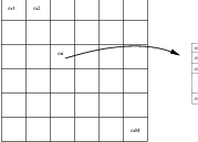
Kohonen’s SOM is usually represented as an array of cells where each cell is, i, associated to a feature (or
weight) vector mi = ![[mi1,mi2,⋅⋅⋅,min]](SoftwareGuide358x.png) T ∈ℝn (figure 19.3).
T ∈ℝn (figure 19.3).
A cell (or neuron) in the map is a good detector for a given input vector x = ![[x1,x2,⋅⋅⋅,xn]](SoftwareGuide360x.png) T ∈ℝn
if the latter is close to the former. This distance between vectors can be represented by the
scalar product xT ⋅mi, but for most of the cases other distances can be used, as for instance
the Euclidean one. The cell having the weight vector closest to the input vector is called the
winner.
T ∈ℝn
if the latter is close to the former. This distance between vectors can be represented by the
scalar product xT ⋅mi, but for most of the cases other distances can be used, as for instance
the Euclidean one. The cell having the weight vector closest to the input vector is called the
winner.
The goal of the learning step is to get a map which is representative of an input example set. It is an iterative
procedure which consists in passing each input example to the map, testing the response of each neuron and
modifying the map to get it closer to the examples.
Algorithm 1 SOM learning:
- t = 0.
- Initialize the weight vectors of the map (randomly, for instance).
- While t < number of iterations, do:
- k = 0.
- While k < number of examples, do:
- Find the vector mi(t) which minimizes the distance d(xk,mi(t))
- For a neighborhood Nc(t) around the winner cell, apply the transformation:
![mi(t+ 1)= mi(t)+ β(t)[xk(t)- mi(t)]](SoftwareGuide361x.png) | (19.2) |
- k = k+1
- t = t +1.
In 19.2, β(t) is a decreasing function with the geometrical distance to the winner cell. For instance:
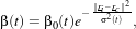 | (19.3) |
with β0(t) and σ(t) decreasing functions with time and r the cell coordinates in the output – map –
space.
Therefore the algorithm consists in getting the map closer to the learning set. The use of a neighborhood
around the winner cell allows the organization of the map into areas which specialize in the recognition of
different patterns. This neighborhood also ensures that cells which are topologically close are also close in
terms of the distance defined in the feature space.
The source code for this example can be found in the file
Examples/Learning/SOMExample.cxx.
This example illustrates the use of the otb::SOM class for building Kohonen’s Self Organizing
Maps.
We will use the SOM in order to build a color table from an input image. Our input image is coded with
3×8 bits and we would like to code it with only 16 levels. We will use the SOM in order to learn which are
the 16 most representative RGB values of the input image and we will assume that this is the optimal color
table for the image.
The first thing to do is include the header file for the class. We will also need the header files for
the map itself and the activation map builder whose utility will be explained at the end of the
example.
#include "otbSOMMap.h" #include "otbSOM.h" #include "otbSOMActivationBuilder.h"
Since the otb::SOM class uses a distance, we will need to include the header file for the one we want to
use
The Self Organizing Map itself is actually an N-dimensional image where each pixel contains a neuron. In
our case, we decide to build a 2-dimensional SOM, where the neurons store RGB values with floating point
precision.
const unsigned int Dimension = 2; typedef double PixelType;
typedef otb::VectorImage<PixelType, Dimension> ImageType;
typedef ImageType::PixelType VectorType;
The distance that we want to apply between the RGB values is the Euclidean one. Of course we
could choose to use other type of distance, as for instance, a distance defined in any other color
space.
typedef itk::Statistics::EuclideanDistanceMetric<VectorType> DistanceType;
We can now define the type for the map. The otb::SOMMap class is templated over the neuron type –
PixelType here –, the distance type and the number of dimensions. Note that the number of dimensions of
the map could be different from the one of the images to be processed.
typedef otb::SOMMap<VectorType, DistanceType, Dimension> MapType;
We are going to perform the learning directly on the pixels of the input image. Therefore, the image type is
defined using the same pixel type as we used for the map. We also define the type for the imge file
reader.
typedef otb::ImageFileReader<ImageType> ReaderType;
Since the otb::SOM class works on lists of samples, it will need to access the input image through an
adaptor. Its type is defined as follows:
typedef itk::Statistics::ListSample<VectorType> SampleListType;
We can now define the type for the SOM, which is templated over the input sample list and the type of the
map to be produced and the two functors that hold the training behavior.
typedef otb::Functor::CzihoSOMLearningBehaviorFunctor LearningBehaviorFunctorType;
typedef otb::Functor::CzihoSOMNeighborhoodBehaviorFunctor
NeighborhoodBehaviorFunctorType; typedef otb::SOM<SampleListType, MapType,
LearningBehaviorFunctorType, NeighborhoodBehaviorFunctorType> SOMType;
As an alternative to standard SOMType, one can decide to use an otb::PeriodicSOM , which behaves like
otb::SOM but is to be considered to as a torus instead of a simple map. Hence, the neighborhood behavior
of the winning neuron does not depend on its location on the map... otb::PeriodicSOM is defined in
otbPeriodicSOM.h.
We can now start building the pipeline. The first step is to instantiate the reader and pass its output to the
adaptor.
ReaderType::Pointer reader = ReaderType::New(); reader->SetFileName(inputFileName);
reader->Update(); SampleListType::Pointer sampleList = SampleListType::New();
sampleList->SetMeasurementVectorSize(reader->GetOutput()->GetVectorLength());
itk::ImageRegionIterator<ImageType> imgIter (reader->GetOutput(),
reader->GetOutput()->
GetBufferedRegion()); imgIter.GoToBegin();
itk::ImageRegionIterator<ImageType> imgIterEnd (reader->GetOutput(),
reader->GetOutput()->
GetBufferedRegion()); imgIterEnd.GoToEnd(); do
{ sampleList->PushBack(imgIter.Get()); ++imgIter; } while (imgIter != imgIterEnd);
We can now instantiate the SOM algorithm and set the sample list as input.
SOMType::Pointer som = SOMType::New(); som->SetListSample(sampleList);
We use a SOMType::SizeType array in order to set the sizes of the map.
SOMType::SizeType size; size[0] = sizeX; size[1] = sizeY; som->SetMapSize(size);
The initial size of the neighborhood of each neuron is set in the same way.
SOMType::SizeType radius; radius[0] = neighInitX; radius[1] = neighInitY;
som->SetNeighborhoodSizeInit(radius);
The other parameters are the number of iterations, the initial and the final values for the learning rate – β –
and the maximum initial value for the neurons (the map will be randomly initialized).
som->SetNumberOfIterations(nbIterations); som->SetBetaInit(betaInit);
som->SetBetaEnd(betaEnd); som->SetMaxWeight(static_cast<PixelType>(initValue));
Now comes the initialization of the functors.
LearningBehaviorFunctorType learningFunctor; learningFunctor.SetIterationThreshold(radius, nbIterations);
som->SetBetaFunctor(learningFunctor); NeighborhoodBehaviorFunctorType neighborFunctor;
som->SetNeighborhoodSizeFunctor(neighborFunctor); som->Update();
Finally, we set up the las part of the pipeline where the plug the output of the SOM into the writer. The
learning procedure is triggered by calling the Update() method on the writer. Since the map is itself an
image, we can write it to disk with an otb::ImageFileWriter .
Figure 19.4 shows the result of the SOM learning. Since we have performed a learning on RGB pixel
values, the produced SOM can be interpreted as an optimal color table for the input image. It can be
observed that the obtained colors are topologically organised, so similar colors are also close in the map.
This topological organisation can be exploited to further reduce the number of coding levels of the pixels
without performing a new learning: we can subsample the map to get a new color table. Also, a
bilinear interpolation between the neurons can be used to increase the number of coding levels.
We can now compute the activation map for the input image. The activation map tells us how many times a
given neuron is activated for the set of examples given to the map. The activation map is stored as a scalar
image and an integer pixel type is usually enough.
typedef unsigned char OutputPixelType; typedef otb::Image<OutputPixelType, Dimension> OutputImageType;
typedef otb::ImageFileWriter<OutputImageType> ActivationWriterType;
In a similar way to the otb::SOM class the otb::SOMActivationBuilder is templated
over the sample list given as input, the SOM map type and the activation map to be built as
output.
typedef otb::SOMActivationBuilder<SampleListType, MapType, OutputImageType> SOMActivationBuilderType;
We instantiate the activation map builder and set as input the SOM map build before and the image (using
the adaptor).
SOMActivationBuilderType::Pointer somAct = SOMActivationBuilderType::New();
somAct->SetInput(som->GetOutput()); somAct->SetListSample(sampleList); somAct->Update();
The final step is to write the activation map to a file.
if (actMapFileName != ITK_NULLPTR) { ActivationWriterType::Pointer actWriter = ActivationWriterType::New();
actWriter->SetFileName(actMapFileName);
The righthand side of figure 19.4 shows the activation map obtained.
The source code for this example can be found in the file
Examples/Learning/SOMClassifierExample.cxx.
This example illustrates the use of the otb::SOMClassifier class for performing a classification using
an existing Kohonen’s Self Organizing. Actually, the SOM classification consists only in the attribution of
the winner neuron index to a given feature vector.
We will use the SOM created in section 19.4.2.1 and we will assume that each neuron represents a class in
the image.
The first thing to do is include the header file for the class.
#include "otbSOMClassifier.h"
As for the SOM learning step, we must define the types for the otb::SOMMap, and therefore, also for
the distance to be used. We will also define the type for the SOM reader, which is actually an
otb::ImageFileReader which the appropriate image type.
typedef itk::Statistics::EuclideanDistanceMetric<PixelType> DistanceType;
typedef otb::SOMMap<PixelType, DistanceType, Dimension> SOMMapType;
typedef otb::ImageFileReader<SOMMapType> SOMReaderType;
The classification will be performed by the otb::SOMClassifier , which, as most of the classifiers,
works on itk::Statistics::ListSample s. In order to be able to perform an image classification, we
will need to use the itk::Statistics::ImageToListAdaptor which is templated over the type of
image to be adapted. The SOMClassifier is templated over the sample type, the SOMMap type and the
pixel type for the labels.
typedef itk::Statistics::ListSample<PixelType> SampleType;
typedef otb::SOMClassifier<SampleType, SOMMapType, LabelPixelType> ClassifierType;
The result of the classification will be stored on an image and saved to a file. Therefore, we define the types
needed for this step.
typedef otb::Image<LabelPixelType, Dimension> OutputImageType;
typedef otb::ImageFileWriter<OutputImageType> WriterType;
We can now start reading the input image and the SOM given as inputs to the program. We instantiate the
readers as usual.
ReaderType::Pointer reader = ReaderType::New(); reader->SetFileName(imageFilename);
reader->Update(); SOMReaderType::Pointer somreader = SOMReaderType::New();
somreader->SetFileName(mapFilename); somreader->Update();
The conversion of the input data from image to list sample is easily done using the adaptor.
SampleType::Pointer sample = SampleType::New(); itk::ImageRegionIterator<InputImageType> it(reader->GetOutput(),
reader->GetOutput()->
GetLargestPossibleRegion());
sample->SetMeasurementVectorSize(reader->GetOutput()->GetNumberOfComponentsPerPixel());
it.GoToBegin(); while (!it.IsAtEnd()) { sample->PushBack(it.Get()); ++it; }
The classifier can now be instantiated. The input data is set by using the SetSample() method and the
SOM si set using the SetMap() method. The classification is triggered by using the Update()
method.
ClassifierType::Pointer classifier = ClassifierType::New(); classifier->SetSample(sample.GetPointer());
classifier->SetMap(somreader->GetOutput()); classifier->Update();
Once the classification has been performed, the sample list obtained at the output of the classifier must be
converted into an image. We create the image as follows :
OutputImageType::Pointer outputImage = OutputImageType::New();
outputImage->SetRegions(reader->GetOutput()->GetLargestPossibleRegion()); outputImage->Allocate();
We can now get a pointer to the classification result.
ClassifierType::OutputType⋆ membershipSample = classifier->GetOutput();
And we can declare the iterators pointing to the front and the back of the sample list.
ClassifierType::OutputType::ConstIterator m_iter = membershipSample->Begin();
ClassifierType::OutputType::ConstIterator m_last = membershipSample->End();
We also declare an itk::ImageRegionIterator in order to fill the output image with the class
labels.
typedef itk::ImageRegionIterator<OutputImageType> OutputIteratorType;
OutputIteratorType outIt(outputImage, outputImage->GetLargestPossibleRegion());
We iterate through the sample list and the output image and assign the label values to the image
pixels.
outIt.GoToBegin(); while (m_iter != m_last && !outIt.IsAtEnd()) {
outIt.Set(m_iter.GetClassLabel()); ++m_iter; ++outIt; }
Finally, we write the classified image to a file.
WriterType::Pointer writer = WriterType::New(); writer->SetFileName(outputFilename);
writer->SetInput(outputImage); writer->Update();
Figure 19.5 shows the result of the SOM classification.
The source code for this example can be found in the file
Examples/Classification/SOMImageClassificationExample.cxx.
In previous examples, we have used the otb::SOMClassifier , which uses the ITK classification
framework. This good for compatibility with the ITK framework, but introduces the limitations
of not being able to use streaming and being able to know at compilation time the number of
bands of the image to be classified. In OTB we have avoided this limitation by developing the
otb::SOMImageClassificationFilter . In this example we will illustrate its use. We start by including
the appropriate header file.
#include "otbSOMImageClassificationFilter.h"
We will assume double precision input images and will also define the type for the labeled
pixels.
const unsigned int Dimension = 2; typedef double PixelType;
typedef unsigned short LabeledPixelType;
Our classifier will be generic enough to be able to process images with any number of bands. We read the
images as otb::VectorImage s. The labeled image will be a scalar image.
typedef otb::VectorImage<PixelType, Dimension> ImageType;
typedef otb::Image<LabeledPixelType, Dimension> LabeledImageType;
We can now define the type for the classifier filter, which is templated over its input and output image types
and the SOM type.
typedef otb::SOMMap<ImageType::PixelType> SOMMapType; typedef otb::SOMImageClassificationFilter<ImageType,
LabeledImageType, SOMMapType> ClassificationFilterType;
And finally, we define the readers (for the input image and theSOM) and the writer. Since the images, to
classify can be very big, we will use a streamed writer which will trigger the streaming ability of the
classifier.
typedef otb::ImageFileReader<ImageType> ReaderType;
typedef otb::ImageFileReader<SOMMapType> SOMReaderType;
typedef otb::ImageFileWriter<LabeledImageType> WriterType;
We instantiate the classifier and the reader objects and we set the existing SOM obtained in a previous
training step.
ClassificationFilterType::Pointer filter = ClassificationFilterType::New();
ReaderType::Pointer reader = ReaderType::New(); reader->SetFileName(infname);
SOMReaderType::Pointer somreader = SOMReaderType::New(); somreader->SetFileName(somfname);
somreader->Update(); filter->SetMap(somreader->GetOutput());
We plug the pipeline and trigger its execution by updating the output of the writer.
filter->SetInput(reader->GetOutput()); WriterType::Pointer writer = WriterType::New();
writer->SetInput(filter->GetOutput()); writer->SetFileName(outfname); writer->Update();
The source code for this example can be found in the file
Examples/Classification/BayesianPluginClassifier.cxx.
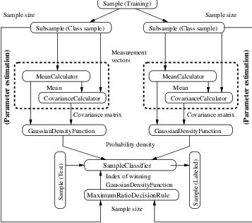
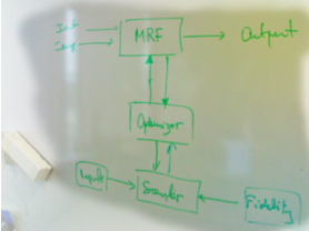
In this example, we present a system that places measurement vectors into two Gaussian classes. The
Figure 19.6 shows all the components of the classifier system and the data flow. This system differs from
the previous k-means clustering algorithms in several ways. The biggest difference is that this classifier
uses the itk::Statistics::GaussianMembershipFunction as membership functions
instead of the itk::Statistics::EuclideanDistanceMetric . Since the membership
function is different, it requires a different set of parameters, mean vectors and covariance
matrices. We choose the itk::Statistics::MeanSampleFilter (sample mean) and the
itk::Statistics::CovarianceSampleFilter (sample covariance) for the estimation algorithms of the
two parameters. If we want a more robust estimation algorithm, we can replace these estimation
algorithms with additional alternatives without changing other components in the classifier
system.
It is a bad idea to use the same sample for both testing and training (parameter estimation) of the
parameters. However, for simplicity, in this example, we use a sample for test and training.
We use the itk::Statistics::ListSample as the sample (test and training). The itk::Vector is our
measurement vector class. To store measurement vectors into two separate sample containers, we use the
itk::Statistics::Subsample objects.
#include "itkVector.h" #include "itkListSample.h" #include "itkSubsample.h"
The following two files provides us with the parameter estimation algorithms.
#include "itkMeanSampleFilter.h" #include "itkCovarianceSampleFilter.h"
The following files define the components required by ITK statistical classification framework: the decision
rule, the membership function, and the classifier.
#include "itkMaximumRatioDecisionRule.h" #include "itkGaussianMembershipFunction.h"
#include "itkSampleClassifierFilter.h"
We will fill the sample with random variables from two normal distributions using the
itk::Statistics::NormalVariateGenerator .
#include "itkNormalVariateGenerator.h"
Since the NormalVariateGenerator class only supports 1-D, we define our measurement vector type as a one
component vector. We then, create a ListSample object for data inputs.
We also create two Subsample objects that will store the measurement vectors in sample into two separate
sample containers. Each Subsample object stores only the measurement vectors belonging to a single class.
This class sample will be used by the parameter estimation algorithms.
typedef itk::Vector<double, 1> MeasurementVectorType;
typedef itk::Statistics::ListSample<MeasurementVectorType> SampleType;
SampleType::Pointer sample = SampleType::New();
sample->SetMeasurementVectorSize(1); // length of measurement vectors
// in the sample. typedef itk::Statistics::Subsample<SampleType> ClassSampleType;
std::vector<ClassSampleType::Pointer> classSamples; for (unsigned int i = 0; i < 2; ++i) {
classSamples.push_back(ClassSampleType::New()); classSamples[i]->SetSample(sample); }
The following code snippet creates a NormalVariateGenerator object. Since the random variable generator
returns values according to the standard normal distribution (the mean is zero, and the standard deviation is
one), before pushing random values into the sample, we change the mean and standard deviation. We need
two normally (Gaussian) distributed datasets. We have two for loops, within which each uses a different
mean and standard deviation. Before we fill the sample with the second distribution data, we call
Initialize(random seed) method, to recreate the pool of random variables in the normalGenerator. In
the second for loop, we fill the two class samples with measurement vectors using the AddInstance()
method.
To see the probability density plots from the two distributions, refer to Figure 19.2.
typedef itk::Statistics::NormalVariateGenerator NormalGeneratorType;
NormalGeneratorType::Pointer normalGenerator = NormalGeneratorType::New();
normalGenerator->Initialize(101); MeasurementVectorType mv;
double mean = 100; double standardDeviation = 30;
SampleType::InstanceIdentifier id = 0UL; for (unsigned int i = 0; i < 100; ++i) {
mv.Fill((normalGenerator->GetVariate() ⋆ standardDeviation) + mean); sample->PushBack(mv);
classSamples[0]->AddInstance(id); ++id; } normalGenerator->Initialize(3024);
mean = 200; standardDeviation = 30; for (unsigned int i = 0; i < 100; ++i)
{ mv.Fill((normalGenerator->GetVariate() ⋆ standardDeviation) + mean);
sample->PushBack(mv); classSamples[1]->AddInstance(id); ++id; }
In the following code snippet, notice that the template argument for the MeanSampleFilter and
CovarianceFilter is ClassSampleType (i.e., type of Subsample) instead of SampleType (i.e. type
of ListSample). This is because the parameter estimation algorithms are applied to the class
sample.
typedef itk::Statistics::MeanSampleFilter<ClassSampleType> MeanEstimatorType;
typedef itk::Statistics::CovarianceSampleFilter<ClassSampleType>
CovarianceEstimatorType; std::vector<MeanEstimatorType::Pointer> meanEstimators;
std::vector<CovarianceEstimatorType::Pointer> covarianceEstimators; for (unsigned int i = 0; i < 2; ++i)
{ meanEstimators.push_back(MeanEstimatorType::New()); meanEstimators[i]->SetInput(classSamples[i]);
meanEstimators[i]->Update(); covarianceEstimators.push_back(CovarianceEstimatorType::New());
covarianceEstimators[i]->SetInput(classSamples[i]);
//covarianceEstimators[i]->SetMean(meanEstimators[i]->GetOutput());
covarianceEstimators[i]->Update(); }
We print out the estimated parameters.
for (unsigned int i = 0; i < 2; ++i) {
std::cout << "class[" << i << "] " << std::endl; std::cout << " estimated mean : "
<< meanEstimators[i]->GetMean() << " covariance matrix : "
<< covarianceEstimators[i]->GetCovarianceMatrixOutput()->Get() << std::endl; }
After creating a SampleClassifierFilter object and a MaximumRatioDecisionRule object, we plug in the
decisionRule and the sample to the classifier. We then specify the number of classes that will be
considered using the SetNumberOfClasses() method.
The MaximumRatioDecisionRule requires a vector of a priori probability values. Such a priori probability
will be the P(ωi) of the following variation of the Bayes decision rule:
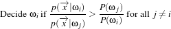 | (19.4) |
The remainder of the code snippet demonstrates how user-specified class labels are used. The classification
result will be stored in a MembershipSample object, and for each measurement vector, its class label will be
one of the two class labels, 100 and 200 (unsigned int).
typedef itk::Statistics::GaussianMembershipFunction <MeasurementVectorType> MembershipFunctionType;
typedef itk::Statistics::MaximumRatioDecisionRule DecisionRuleType;
DecisionRuleType::Pointer decisionRule = DecisionRuleType::New();
DecisionRuleType::PriorProbabilityVectorType aPrioris; aPrioris.push_back(classSamples[0]->GetTotalFrequency()
/ sample->GetTotalFrequency()); aPrioris.push_back(classSamples[1]->GetTotalFrequency()
/ sample->GetTotalFrequency()); decisionRule->SetPriorProbabilities(aPrioris);
typedef itk::Statistics::SampleClassifierFilter<SampleType> ClassifierType;
ClassifierType::Pointer classifier = ClassifierType::New();
classifier->SetDecisionRule(dynamic_cast< itk::Statistics::DecisionRule⋆ >( decisionRule.GetPointer()));
classifier->SetInput(sample); classifier->SetNumberOfClasses(2); std::vector<long unsigned int> classLabels;
classLabels.resize(2); classLabels[0] = 100; classLabels[1] = 200;
typedef itk::SimpleDataObjectDecorator<std::vector<long unsigned int> > ClassLabelDecoratedType;
ClassLabelDecoratedType::Pointer classLabelsDecorated = ClassLabelDecoratedType::New();
classLabelsDecorated->Set(classLabels); classifier->SetClassLabels(classLabelsDecorated);
The classifier is almost ready to perform the classification except that it needs two membership
functions that represent the two clusters.
In this example, we can imagine that the two clusters are modeled by two Euclidean distance functions. The
distance function (model) has only one parameter, the mean (centroid) set by the SetOrigin() method. To
plug-in two distance functions, we call the AddMembershipFunction() method. Finally, the invocation of
the Update() method will perform the classification.
typedef ClassifierType::MembershipFunctionType MembershipFunctionBaseType;
typedef ClassifierType::MembershipFunctionVectorObjectType::ComponentType ComponentMembershipType;
// Vector Containing the membership function used
ComponentMembershipType membershipFunctions; for (unsigned int i = 0; i < 2; i++)
{ MembershipFunctionType::Pointer curMemshpFunction = MembershipFunctionType::New();
curMemshpFunction->SetMean(meanEstimators[i]->GetMean());
curMemshpFunction->SetCovariance(covarianceEstimators[i]->GetCovarianceMatrix());
// cast the GaussianMembershipFunction in a // itk::MembershipFunctionBase
membershipFunctions.push_back(dynamic_cast<const MembershipFunctionBaseType⋆ >(curMemshpFunction.GetPointer()));
}
ClassifierType::MembershipFunctionVectorObjectPointer membershipVectorObject = ClassifierType::MembershipFunctionVectorObjectType::New();
membershipVectorObject->Set(membershipFunctions);
classifier->SetMembershipFunctions(membershipVectorObject); classifier->Update();
The following code snippet prints out pairs of a measurement vector and its class label in the
sample.
const ClassifierType::MembershipSampleType⋆ membershipSample = classifier->GetOutput();
ClassifierType::MembershipSampleType::ConstIterator iter = membershipSample->Begin();
while (iter != membershipSample->End()) { std::cout << "measurement vector = " << iter.GetMeasurementVector()
<< "class label = " << iter.GetClassLabel() << std::endl; ++iter; }
The source code for this example can be found in the file
Examples/Classification/ExpectationMaximizationMixtureModelEstimator.cxx.
In this example, we present ITK’s implementation of the expectation maximization (EM) process to
generate parameter estimates for a two Gaussian component mixture model.
The Bayesian plug-in classifier example (see Section 19.4.3) used two Gaussian probability density
functions (PDF) to model two Gaussian distribution classes (two models for two class). However, in
some cases, we want to model a distribution as a mixture of several different distributions.
Therefore, the probability density function (p(x)) of a mixture model can be stated as follows
:
 | (19.5) |
where i is the index of the component, c is the number of components, αi is the proportion of the
component, and fi is the probability density function of the component.
Now the task is to find the parameters(the component PDF’s parameters and the proportion values) to
maximize the likelihood of the parameters. If we know which component a measurement vector belongs to,
the solutions to this problem is easy to solve. However, we don’t know the membership of each
measurement vector. Therefore, we use the expectation of membership instead of the exact membership.
The EM process splits into two steps:
- E step: calculate the expected membership values for each measurement vector to each
classes.
- M step: find the next parameter sets that maximize the likelihood with the expected
membership values and the current set of parameters.
The E step is basically a step that calculates the a posteriori probability for each measurement
vector.
The M step is dependent on the type of each PDF. Most of distributions belonging to exponential family
such as Poisson, Binomial, Exponential, and Normal distributions have analytical solutions for updating the
parameter set. The itk::Statistics::ExpectationMaximizationMixtureModelEstimator class
assumes that such type of components.
In the following example we use the itk::Statistics::ListSample as the sample (test and training).
The itk::Vector is our measurement vector class. To store measurement vectors into two separate
sample container, we use the itk::Statistics::Subsample objects.
#include "itkVector.h" #include "itkListSample.h"
The following two files provide us the parameter estimation algorithms.
#include "itkGaussianMixtureModelComponent.h"
#include "itkExpectationMaximizationMixtureModelEstimator.h"
We will fill the sample with random variables from two normal distribution using the
itk::Statistics::NormalVariateGenerator .
#include "itkNormalVariateGenerator.h"
Since the NormalVariateGenerator class only supports 1-D, we define our measurement vector type as a one
component vector. We then, create a ListSample object for data inputs.
We also create two Subsample objects that will store the measurement vectors in the sample into two
separate sample containers. Each Subsample object stores only the measurement vectors belonging to a
single class. This class sample will be used by the parameter estimation algorithms.
unsigned int numberOfClasses = 2; typedef itk::Vector<double, 1>
MeasurementVectorType; typedef itk::Statistics::ListSample<MeasurementVectorType> SampleType;
SampleType::Pointer sample = SampleType::New();
sample->SetMeasurementVectorSize(1); // length of measurement vectors // in the sample.
The following code snippet creates a NormalVariateGenerator object. Since the random variable generator
returns values according to the standard normal distribution (the mean is zero, and the standard deviation is
one) before pushing random values into the sample, we change the mean and standard deviation. We want
two normal (Gaussian) distribution data. We have two for loops. Each for loop uses different mean
and standard deviation. Before we fill the sample with the second distribution data, we call
Initialize() method to recreate the pool of random variables in the normalGenerator. In the second
for loop, we fill the two class samples with measurement vectors using the AddInstance()
method.
To see the probability density plots from the two distribution, refer to Figure 19.2.
typedef itk::Statistics::NormalVariateGenerator NormalGeneratorType;
NormalGeneratorType::Pointer normalGenerator = NormalGeneratorType::New();
normalGenerator->Initialize(101); MeasurementVectorType mv; double mean = 100;
double standardDeviation = 30; for (unsigned int i = 0; i < 100; ++i)
{ mv[0] = (normalGenerator->GetVariate() ⋆ standardDeviation) + mean;
sample->PushBack(mv); } normalGenerator->Initialize(3024); mean = 200;
standardDeviation = 30; for (unsigned int i = 0; i < 100; ++i) {
mv[0] = (normalGenerator->GetVariate() ⋆ standardDeviation) + mean; sample->PushBack(mv); }
In the following code snippet notice that the template argument for the MeanSampleFilter and
CovarianceSampleFilter is ClassSampleType (i.e., type of Subsample) instead of SampleType (i.e., type
of ListSample). This is because the parameter estimation algorithms are applied to the class
sample.
typedef itk::Array<double> ParametersType; ParametersType params(2);
std::vector<ParametersType> initialParameters(numberOfClasses); params[0] = 110.0;
params[1] = 800.0; initialParameters[0] = params; params[0] = 210.0; params[1] = 850.0;
initialParameters[1] = params; typedef itk::Statistics::GaussianMixtureModelComponent<SampleType>
ComponentType; std::vector<ComponentType::Pointer> components;
for (unsigned int i = 0; i < numberOfClasses; ++i) { components.push_back(ComponentType::New());
(components[i])->SetSample(sample); (components[i])->SetParameters(initialParameters[i]); }
We run the estimator.
typedef itk::Statistics::ExpectationMaximizationMixtureModelEstimator< SampleType> EstimatorType;
EstimatorType::Pointer estimator = EstimatorType::New(); estimator->SetSample(sample);
estimator->SetMaximumIteration(200); itk::Array<double> initialProportions(numberOfClasses);
initialProportions[0] = 0.5; initialProportions[1] = 0.5;
estimator->SetInitialProportions(initialProportions); for (unsigned int i = 0; i < numberOfClasses; ++i)
{ estimator->AddComponent((ComponentType::Superclass⋆)
(components[i]).GetPointer()); } estimator->Update();
We then print out the estimated parameters.
for (unsigned int i = 0; i < numberOfClasses; ++i) {
std::cout << "Cluster[" << i << "]" << std::endl; std::cout << " Parameters:" << std::endl;
std::cout << " " << (components[i])->GetFullParameters()
<< std::endl; std::cout << " Proportion: ";
std::cout << " " << (estimator->GetProportions())[i] << std::endl; }
The Stochastic Expectation Maximization (SEM) approach is a stochastic version of the EM mixture
estimation seen on section 19.4.4. It has been introduced by [22] to prevent convergence of the EM
approach from local minima. It avoids the analytical maximization issued by integrating a stochastic
sampling procedure in the estimation process. It induces an almost sure (a.s.) convergence to the
algorithm.
From the initial two step formulation of the EM mixture estimation, the SEM may be decomposed into 3
steps:
- E-step, calculates the expected membership values for each measurement vector to each
classes.
- S-step, performs a stochastic sampling of the membership vector to each classes, according
to the membership values computed in the E-step.
- M-step, updates the parameters of the membership probabilities (parameters to be defined
through the class itk::Statistics::ModelComponentBase and its inherited classes).
The implementation of the SEM has been turned to a contextual SEM in the sense where the evaluation of
the membership parameters is conditioned to membership values of the spatial neighborhood of each
pixels.
The source code for this example can be found in the file
Examples/Learning/SEMModelEstimatorExample.cxx.
In this example, we present OTB’s implementation of SEM, through the class otb::SEMClassifier .
This class performs a stochastic version of the EM algorithm, but instead of inheriting from
itk::ExpectationMaximizationMixtureModelEstimator , we chose to inherit from
itk::Statistics::ListSample , in the same way as otb::SVMClassifier .
The program begins with otb::VectorImage and outputs otb::Image . Then appropriate header files
have to be included:
#include "otbImage.h" #include "otbVectorImage.h" #include "otbImageFileReader.h"
#include "otbImageFileWriter.h"
otb::SEMClassifier performs estimation of mixture to fit the initial histogram. Actually, mixture of
Gaussian pdf can be performed. Those generic pdf are treated in otb::Statistics::ModelComponentBase .
The Gaussian model is taken in charge with the class otb::Statistics::GaussianModelComponent
.
#include "otbSEMClassifier.h"
Input/Output images type are define in a classical way. In fact, a itk::VariableLengthVector is to be
considered for the templated MeasurementVectorType, which will be used in the ListSample
interface.
typedef double PixelType; typedef otb::VectorImage<PixelType, 2> ImageType;
typedef otb::ImageFileReader<ImageType> ReaderType;
typedef otb::Image<unsigned char, 2> OutputImageType;
typedef otb::ImageFileWriter<OutputImageType> WriterType;
Once the input image is opened, the classifier may be initialised by SmartPointer.
typedef otb::SEMClassifier<ImageType, OutputImageType> ClassifType;
ClassifType::Pointer classifier = ClassifType::New();
Then, it follows, classical initializations of the pipeline.
classifier->SetNumberOfClasses(numberOfClasses); classifier->SetMaximumIteration(numberOfIteration);
classifier->SetNeighborhood(neighborhood); classifier->SetTerminationThreshold(terminationThreshold);
classifier->SetSample(reader->GetOutput());
When an initial segmentation is available, the classifier may use it as image (of type OutputImageType) or
as a itk::SampleClassifier result (of type itk::Statistics::MembershipSample ).
if (fileNameImgInit != ITK_NULLPTR) { typedef otb::ImageFileReader<OutputImageType> ImgInitReaderType;
ImgInitReaderType::Pointer segReader = ImgInitReaderType::New(); segReader->SetFileName(fileNameImgInit);
segReader->Update(); classifier->SetClassLabels(segReader->GetOutput()); }
By default, otb::SEMClassifier performs initialization of ModelComponentBase by as many
instantiation of otb::Statistics::GaussianModelComponent as the number of classes to estimate in
the mixture. Nevertheless, the user may add specific distribution into the mixture estimation. It is
permitted by the use of AddComponent for the given class number and the specific distribution.
typedef ClassifType::ClassSampleType ClassSampleType;
typedef otb::Statistics::GaussianModelComponent<ClassSampleType>
GaussianType; for (int i = 0; i < numberOfClasses; ++i) {
GaussianType::Pointer model = GaussianType::New(); classifier->AddComponent(i, model); }
Once the pipeline is instantiated. The segmentation by itself may be launched by using the Update function.
try { classifier->Update(); }
The segmentation may outputs a result of type itk::Statistics::MembershipSample as it is the case
for the otb::SVMClassifier . But when using GetOutputImage the output is directly an
Image.
Only for visualization purposes, we choose to rescale the image of classes before saving it to a file. We will
use the itk::RescaleIntensityImageFilter for this purpose.
typedef itk::RescaleIntensityImageFilter<OutputImageType,
OutputImageType> RescalerType; RescalerType::Pointer rescaler = RescalerType::New();
rescaler->SetOutputMinimum(itk::NumericTraits<unsigned char>::min());
rescaler->SetOutputMaximum(itk::NumericTraits<unsigned char>::max());
rescaler->SetInput(classifier->GetOutputImage()); WriterType::Pointer writer = WriterType::New();
writer->SetFileName(fileNameOut); writer->SetInput(rescaler->GetOutput()); writer->Update();
Figure 19.7 shows the result of the SEM segmentation with 4 different classes and a contextual
neighborhood of 3 pixels.
As soon as the segmentation is performed by an iterative stochastic process, it is worth verifying the output
status: does the segmentation ends when it has converged or just at the limit of the iteration
numbers.
std::cerr << "Program terminated with a "; if (classifier->GetTerminationCode() ==
ClassifType::CONVERGED) std::cerr << "converged "; else std::cerr << "not-converged ";
std::cerr << "code...\n";
The text output gives for each class the parameters of the pdf (e.g. mean of each component of the class and
there covariance matrix, in the case of a Gaussian mixture model).
classifier->Print(std::cerr);
Markov Random Fields are probabilistic models that use the statistical dependency between pixels in a
neighborhood to infeer the value of a give pixel.
The itk::Statistics::MRFImageFilter uses the maximum a posteriori (MAP) estimates
for modeling the MRF. The object traverses the data set and uses the model generated by the
Mahalanobis distance classifier to get the the distance between each pixel in the data set to
a set of known classes, updates the distances by evaluating the influence of its neighboring
pixels (based on a MRF model) and finally, classifies each pixel to the class which has the
minimum distance to that pixel (taking the neighborhood influence under consideration). The
energy function minimization is done using the iterated conditional modes (ICM) algorithm
[12].
The source code for this example can be found in the file
Examples/Classification/ScalarImageMarkovRandomField1.cxx.
This example shows how to use the Markov Random Field approach for classifying the pixel of a scalar
image.
The itk::Statistics::MRFImageFilter is used for refining an initial classification by introducing the
spatial coherence of the labels. The user should provide two images as input. The first image is
the one to be classified while the second image is an image of labels representing an initial
classification.
The following headers are related to reading input images, writing the output image, and making the
necessary conversions between scalar and vector images.
#include "otbImage.h" #include "itkFixedArray.h" #include "otbImageFileReader.h"
#include "otbImageFileWriter.h" #include "itkComposeImageFilter.h"
The following headers are related to the statistical classification classes.
#include "itkMRFImageFilter.h" #include "itkDistanceToCentroidMembershipFunction.h"
#include "itkMinimumDecisionRule.h"
First we define the pixel type and dimension of the image that we intend to classify. With this image type
we can also declare the otb::ImageFileReader needed for reading the input image, create one and set
its input filename.
typedef unsigned char PixelType; const unsigned int Dimension = 2;
typedef otb::Image<PixelType, Dimension> ImageType; typedef otb::ImageFileReader<ImageType> ReaderType;
ReaderType::Pointer reader = ReaderType::New(); reader->SetFileName(inputImageFileName);
As a second step we define the pixel type and dimension of the image of labels that provides the initial
classification of the pixels from the first image. This initial labeled image can be the output of a K-Means
method like the one illustrated in section 19.4.1.
typedef unsigned char LabelPixelType; typedef otb::Image<LabelPixelType, Dimension> LabelImageType;
typedef otb::ImageFileReader<LabelImageType> LabelReaderType;
LabelReaderType::Pointer labelReader = LabelReaderType::New(); labelReader->SetFileName(inputLabelImageFileName);
Since the Markov Random Field algorithm is defined in general for images whose pixels have multiple
components, that is, images of vector type, we must adapt our scalar image in order to satisfy the interface
expected by the MRFImageFilter. We do this by using the itk::ScalarToArrayCastImageFilter .
With this filter we will present our scalar image as a vector image whose vector pixels contain a single
component.
typedef itk::FixedArray<LabelPixelType, 1> ArrayPixelType;
typedef otb::Image<ArrayPixelType, Dimension> ArrayImageType; typedef itk::ComposeImageFilter<
ImageType, ArrayImageType> ScalarToArrayFilterType; ScalarToArrayFilterType::Pointer
scalarToArrayFilter = ScalarToArrayFilterType::New(); scalarToArrayFilter->SetInput(0, reader->GetOutput());
With the input image type ImageType and labeled image type LabelImageType we instantiate the type of
the itk::MRFImageFilter that will apply the Markov Random Field algorithm in order to refine the
pixel classification.
typedef itk::MRFImageFilter<ArrayImageType, LabelImageType> MRFFilterType;
MRFFilterType::Pointer mrfFilter = MRFFilterType::New(); mrfFilter->SetInput(scalarToArrayFilter->GetOutput());
We set now some of the parameters for the MRF filter. In particular, the number of classes to be used during
the classification, the maximum number of iterations to be run in this filter and the error tolerance that will
be used as a criterion for convergence.
mrfFilter->SetNumberOfClasses(numberOfClasses); mrfFilter->SetMaximumNumberOfIterations(numberOfIterations);
mrfFilter->SetErrorTolerance(1e-7);
The smoothing factor represents the tradeoff between fidelity to the observed image and the smoothness of
the segmented image. Typical smoothing factors have values between 1 5. This factor will
multiply the weights that define the influence of neighbors on the classification of a given pixel.
The higher the value, the more uniform will be the regions resulting from the classification
refinement.
mrfFilter->SetSmoothingFactor(smoothingFactor);
Given that the MRF filter needs to continually relabel the pixels, it needs access to a set of membership
functions that will measure to what degree every pixel belongs to a particular class. The classification is
performed by the itk::ImageClassifierBase class, that is instantiated using the type of the input
vector image and the type of the labeled image.
typedef itk::ImageClassifierBase< ArrayImageType, LabelImageType> SupervisedClassifierType;
SupervisedClassifierType::Pointer classifier = SupervisedClassifierType::New();
The classifier needs a decision rule to be set by the user. Note that we must use GetPointer() in the call of
the SetDecisionRule() method because we are passing a SmartPointer, and smart pointer cannot perform
polymorphism, we must then extract the raw pointer that is associated to the smart pointer. This extraction
is done with the GetPointer() method.
typedef itk::Statistics::MinimumDecisionRule DecisionRuleType;
DecisionRuleType::Pointer classifierDecisionRule = DecisionRuleType::New();
classifier->SetDecisionRule(classifierDecisionRule.GetPointer());
We now instantiate the membership functions. In this case we use the
itk::Statistics::DistanceToCentroidMembershipFunction class templated over the pixel type of
the vector image, which in our example happens to be a vector of dimension 1.
typedef itk::Statistics::DistanceToCentroidMembershipFunction< ArrayPixelType> MembershipFunctionType;
typedef MembershipFunctionType::Pointer MembershipFunctionPointer; double meanDistance = 0;
MembershipFunctionType::CentroidType centroid(reader->GetOutput()->GetNumberOfComponentsPerPixel());
for (unsigned int i = 0; i < numberOfClasses; ++i) {
MembershipFunctionPointer membershipFunction = MembershipFunctionType::New();
membershipFunction->SetMeasurementVectorSize(reader->GetOutput()->GetNumberOfComponentsPerPixel());
centroid[0] = atof(argv[i + numberOfArgumentsBeforeMeans]);
membershipFunction->SetCentroid(centroid); classifier->AddMembershipFunction(membershipFunction);
meanDistance += static_cast<double> (centroid[0]); } meanDistance /= numberOfClasses;
and we set the neighborhood radius that will define the size of the clique to be used in the computation of
the neighbors’ influence in the classification of any given pixel. Note that despite the fact that we call this a
radius, it is actually the half size of an hypercube. That is, the actual region of influence will not be circular
but rather an N-Dimensional box. For example, a neighborhood radius of 2 in a 3D image will
result in a clique of size 5x5x5 pixels, and a radius of 1 will result in a clique of size 3x3x3
pixels.
mrfFilter->SetNeighborhoodRadius(1);
We should now set the weights used for the neighbors. This is done by passing an array of values that
contains the linear sequence of weights for the neighbors. For example, in a neighborhood of
size 3x3x3, we should provide a linear array of 9 weight values. The values are packaged in a
std::vector and are supposed to be double. The following lines illustrate a typical set of values for a
3x3x3 neighborhood. The array is arranged and then passed to the filter by using the method
SetMRFNeighborhoodWeight().
std::vector<double> weights; weights.push_back(1.5); weights.push_back(2.0); weights.push_back(1.5);
weights.push_back(2.0); weights.push_back(0.0); // This is the central pixel
weights.push_back(2.0); weights.push_back(1.5); weights.push_back(2.0); weights.push_back(1.5);
We now scale weights so that the smoothing function and the image fidelity functions have
comparable value. This is necessary since the label image and the input image can have different
dynamic ranges. The fidelity function is usually computed using a distance function, such as the
itk::DistanceToCentroidMembershipFunction or one of the other membership functions. They tend
to have values in the order of the means specified.
double totalWeight = 0; for (std::vector<double>::const_iterator wcIt = weights.begin();
wcIt != weights.end(); ++wcIt) { totalWeight += ⋆wcIt; }
for (std::vector<double>::iterator wIt = weights.begin(); wIt != weights.end(); wIt++)
{ ⋆wIt = static_cast<double> ((⋆wIt) ⋆ meanDistance / (2 ⋆ totalWeight)); }
mrfFilter->SetMRFNeighborhoodWeight(weights);
Finally, the classifier class is connected to the Markov Random Fields filter.
mrfFilter->SetClassifier(classifier);
The output image produced by the itk::MRFImageFilter has the same pixel type as the
labeled input image. In the following lines we use the OutputImageType in order to instantiate
the type of a otb::ImageFileWriter . Then create one, and connect it to the output of the
classification filter after passing it through an intensity rescaler to rescale it to an 8 bit dynamic
range
typedef MRFFilterType::OutputImageType OutputImageType;
typedef otb::ImageFileWriter<OutputImageType> WriterType; WriterType::Pointer writer = WriterType::New();
writer->SetInput(intensityRescaler->GetOutput()); writer->SetFileName(outputImageFileName);
We are now ready for triggering the execution of the pipeline. This is done by simply invoking the
Update() method in the writer. This call will propagate the update request to the reader and then to the
MRF filter.
try { writer->Update(); } catch (itk::ExceptionObject& excp) {
std::cerr << "Problem encountered while writing "; std::cerr << " image file : " << argv[2] << std::endl;
std::cerr << excp << std::endl; return EXIT_FAILURE; }
Figure 19.8 illustrates the effect of this filter with four classes. In this example the filter was run with a
smoothing factor of 3. The labeled image was produced by ScalarImageKmeansClassifier.cxx and the
means were estimated by ScalarImageKmeansModelEstimator.cxx described in section 19.4.1. The
obtained result can be compared with the one of figure 19.1 to see the interest of using the MRF approach
in order to ensure the regularization of the classified image.
The ITK approach was considered not to be flexible enough for some remote sensing applications.
Therefore, we decided to implement our own framework.
The source code for this example can be found in the file
Examples/Markov/MarkovClassification1Example.cxx.
This example illustrates the details of the otb::MarkovRandomFieldFilter . This filter is an application
of the Markov Random Fields for classification, segmentation or restoration.
This example applies the otb::MarkovRandomFieldFilter to classify an image into four classes
defined by their mean and variance. The optimization is done using an Metropolis algorithm with a random
sampler. The regularization energy is defined by a Potts model and the fidelity by a Gaussian
model.
The first step toward the use of this filter is the inclusion of the proper header files.
#include "otbMRFEnergyPotts.h" #include "otbMRFEnergyGaussianClassification.h"
#include "otbMRFOptimizerMetropolis.h" #include "otbMRFSamplerRandom.h"
Then we must decide what pixel type to use for the image. We choose to make all computations with
double precision. The labelled image is of type unsigned char which allows up to 256 different
classes.
const unsigned int Dimension = 2; typedef double InternalPixelType;
typedef unsigned char LabelledPixelType;
typedef otb::Image<InternalPixelType, Dimension> InputImageType;
typedef otb::Image<LabelledPixelType, Dimension> LabelledImageType;
We define a reader for the image to be classified, an initialization for the classification (which could be
random) and a writer for the final classification.
typedef otb::ImageFileReader<InputImageType> ReaderType;
typedef otb::ImageFileWriter<LabelledImageType> WriterType;
ReaderType::Pointer reader = ReaderType::New(); WriterType::Pointer writer = WriterType::New();
const char ⋆ inputFilename = argv[1]; const char ⋆ outputFilename = argv[2];
reader->SetFileName(inputFilename); writer->SetFileName(outputFilename);
Finally, we define the different classes necessary for the Markov classification. A
otb::MarkovRandomFieldFilter is instantiated, this is the main class which connect the other to do the
Markov classification.
typedef otb::MarkovRandomFieldFilter <InputImageType, LabelledImageType> MarkovRandomFieldFilterType;
An otb::MRFSamplerRandomMAP , which derives from the otb::MRFSampler , is instantiated. The
sampler is in charge of proposing a modification for a given site. The otb::MRFSamplerRandomMAP ,
randomly pick one possible value according to the MAP probability.
typedef otb::MRFSamplerRandom<InputImageType, LabelledImageType> SamplerType;
An otb::MRFOptimizerMetropoli , which derives from the otb::MRFOptimizer , is instantiated.
The optimizer is in charge of accepting or rejecting the value proposed by the sampler. The
otb::MRFSamplerRandomMAP , accept the proposal according to the variation of energy it causes and a
temperature parameter.
typedef otb::MRFOptimizerMetropolis OptimizerType;
Two energy, deriving from the otb::MRFEnergy class need to be instantiated. One energy is required for
the regularization, taking into account the relashionship between neighborhing pixels in the
classified image. Here it is done with the otb::MRFEnergyPotts which implement a Potts
model.
The second energy is for the fidelity to the original data. Here it is done with an
otb::MRFEnergyGaussianClassification class, which defines a gaussian model for the
data.
typedef otb::MRFEnergyPotts <LabelledImageType, LabelledImageType> EnergyRegularizationType;
typedef otb::MRFEnergyGaussianClassification <InputImageType, LabelledImageType> EnergyFidelityType;
The different filters composing our pipeline are created by invoking their New() methods, assigning the
results to smart pointers.
MarkovRandomFieldFilterType::Pointer markovFilter = MarkovRandomFieldFilterType::New();
EnergyRegularizationType::Pointer energyRegularization = EnergyRegularizationType::New();
EnergyFidelityType::Pointer energyFidelity = EnergyFidelityType::New();
OptimizerType::Pointer optimizer = OptimizerType::New();
SamplerType::Pointer sampler = SamplerType::New();
Parameter for the otb::MRFEnergyGaussianClassification class, meand and standard deviation are
created.
unsigned int nClass = 4; energyFidelity->SetNumberOfParameters(2 ⋆ nClass);
EnergyFidelityType::ParametersType parameters; parameters.SetSize(energyFidelity->GetNumberOfParameters());
parameters[0] = 10.0; //Class 0 mean parameters[1] = 10.0; //Class 0 stdev
parameters[2] = 80.0; //Class 1 mean parameters[3] = 10.0; //Class 1 stdev
parameters[4] = 150.0; //Class 2 mean parameters[5] = 10.0; //Class 2 stdev
parameters[6] = 220.0; //Class 3 mean parameters[7] = 10.0; //Class 3 stde
energyFidelity->SetParameters(parameters);
Parameters are given to the different class an the sampler, optimizer and energies are connected with the
Markov filter.
OptimizerType::ParametersType param(1); param.Fill(atof(argv[5])); optimizer->SetParameters(param);
markovFilter->SetNumberOfClasses(nClass); markovFilter->SetMaximumNumberOfIterations(atoi(argv[4]));
markovFilter->SetErrorTolerance(0.0); markovFilter->SetLambda(atof(argv[3]));
markovFilter->SetNeighborhoodRadius(1); markovFilter->SetEnergyRegularization(energyRegularization);
markovFilter->SetEnergyFidelity(energyFidelity); markovFilter->SetOptimizer(optimizer);
markovFilter->SetSampler(sampler);
The pipeline is connected. An itk::RescaleIntensityImageFilter rescale the classified image before
saving it.
markovFilter->SetInput(reader->GetOutput()); typedef itk::RescaleIntensityImageFilter
<LabelledImageType, LabelledImageType> RescaleType; RescaleType::Pointer rescaleFilter = RescaleType::New();
rescaleFilter->SetOutputMinimum(0); rescaleFilter->SetOutputMaximum(255);
rescaleFilter->SetInput(markovFilter->GetOutput()); writer->SetInput(rescaleFilter->GetOutput());
Finally, the pipeline execution is trigerred.
Figure 19.10 shows the output of the Markov Random Field classification after 20 iterations with a random
sampler and a Metropolis optimizer.
The source code for this example can be found in the file
Examples/Markov/MarkovClassification2Example.cxx.
Using a similar structure as the previous program and the same energy function, we are now going to
slightly alter the program to use a different sampler and optimizer. The proposed sample is proposed
randomly according to the MAP probability and the optimizer is the ICM which accept the proposed
sample if it enable a reduction of the energy.
First, we need to include header specific to these class:
#include "otbMRFSamplerRandomMAP.h" #include "otbMRFOptimizerICM.h"
And to declare these new type:
typedef otb::MRFSamplerRandomMAP<InputImageType, LabelledImageType> SamplerType;
// typedef otb::MRFSamplerRandom< InputImageType, LabelledImageType> SamplerType;
typedef otb::MRFOptimizerICM OptimizerType;
As the otb::MRFOptimizerICM does not have any parameters, the call to optimizer->SetParameters()
must be removed
Apart from these, no further modification is required.
Figure 19.11 shows the output of the Markov Random Field classification after 5 iterations with a MAP
random sampler and an ICM optimizer.
The source code for this example can be found in the file
Examples/Markov/MarkovClassification3Example.cxx.
This example illustrates the details of the MarkovRandomFieldFilter by using the Fisher distribution to
model the likelihood energy. This filter is an application of the Markov Random Fields for
classification.
This example applies the MarkovRandomFieldFilter to classify an image into four classes defined by their
Fisher distribution parameters L, M and mu. The optimization is done using a Metropolis algorithm with a
random sampler. The regularization energy is defined by a Potts model and the fidelity or likelihood energy
is modelled by a Fisher distribution. The parameter of the Fisher distribution was determined for each class
in a supervised step. ( See the File OtbParameterEstimatioOfFisherDistribution ) This example is a
contribution from Jan Wegner.
Then we must decide what pixel type to use for the image. We choose to make all computations with
double precision. The labeled image is of type unsigned char which allows up to 256 different
classes.
const unsigned int Dimension = 2; typedef double InternalPixelType;
typedef unsigned char LabelledPixelType; typedef otb::Image<InternalPixelType, Dimension> InputImageType;
typedef otb::Image<LabelledPixelType, Dimension> LabelledImageType;
We define a reader for the image to be classified, an initialization for the classification (which could be
random) and a writer for the final classification.
typedef otb::ImageFileReader< InputImageType > ReaderType;
typedef otb::ImageFileWriter< LabelledImageType > WriterType;
ReaderType::Pointer reader = ReaderType::New(); WriterType::Pointer writer = WriterType::New();
Finally, we define the different classes necessary for the Markov classification. A MarkovRandomFieldFilter is
instantiated, this is the main class which connect the other to do the Markov classification.
typedef otb::MarkovRandomFieldFilter <InputImageType, LabelledImageType> MarkovRandomFieldFilterType;
An MRFSamplerRandomMAP, which derives from the MRFSampler, is instantiated. The sampler is in
charge of proposing a modification for a given site. The MRFSamplerRandomMAP, randomly pick one
possible value according to the MAP probability.
typedef otb::MRFSamplerRandom< InputImageType, LabelledImageType> SamplerType;
An MRFOptimizerMetropolis, which derives from the MRFOptimizer, is instantiated. The optimizer is in
charge of accepting or rejecting the value proposed by the sampler. The MRFSamplerRandomMAP, accept
the proposal according to the variation of energy it causes and a temperature parameter.
typedef otb::MRFOptimizerMetropolis OptimizerType;
Two energy, deriving from the MRFEnergy class need to be instantiated. One energy is required for the
regularization, taking into account the relationship between neighboring pixels in the classified image. Here
it is done with the MRFEnergyPotts, which implements a Potts model.
The second energy is used for the fidelity to the original data. Here it is done with a
MRFEnergyFisherClassification class, which defines a Fisher distribution to model the data.
typedef otb::MRFEnergyPotts <LabelledImageType, LabelledImageType> EnergyRegularizationType;
typedef otb::MRFEnergyFisherClassification <InputImageType, LabelledImageType> EnergyFidelityType;
The different filters composing our pipeline are created by invoking their New() methods, assigning the
results to smart pointers.
MarkovRandomFieldFilterType::Pointer markovFilter = MarkovRandomFieldFilterType::New();
EnergyRegularizationType::Pointer energyRegularization = EnergyRegularizationType::New();
EnergyFidelityType::Pointer energyFidelity = EnergyFidelityType::New();
OptimizerType::Pointer optimizer = OptimizerType::New(); SamplerType::Pointer sampler = SamplerType::New();
Parameter for the MRFEnergyFisherClassification class are created. The shape parameters M, L and the
weighting parameter mu are computed in a supervised step
unsigned int nClass =4; energyFidelity->SetNumberOfParameters(3⋆nClass);
EnergyFidelityType::ParametersType parameters; parameters.SetSize(energyFidelity->GetNumberOfParameters());
//Class 0 parameters[0] = 12.353042; //Class 0 mu
parameters[1] = 2.156422; //Class 0 L parameters[2] = 4.920403; //Class 0 M
//Class 1 parameters[3] = 72.068291; //Class 1 mu
parameters[4] = 11.000000; //Class 1 L parameters[5] = 50.950001; //Class 1 M
//Class 2 parameters[6] = 146.665985; //Class 2 mu
parameters[7] = 11.000000; //Class 2 L parameters[8] = 50.900002; //Class 2 M
//Class 3 parameters[9] = 200.010132; //Class 3 mu
parameters[10] = 11.000000; //Class 3 L parameters[11] = 50.950001; //Class 3 M
energyFidelity->SetParameters(parameters);
Parameters are given to the different classes and the sampler, optimizer and energies are connected with the
Markov filter.
OptimizerType::ParametersType param(1); param.Fill(atof(argv[6])); optimizer->SetParameters(param);
markovFilter->SetNumberOfClasses(nClass); markovFilter->SetMaximumNumberOfIterations(atoi(argv[5]));
markovFilter->SetErrorTolerance(0.0); markovFilter->SetLambda(atof(argv[4]));
markovFilter->SetNeighborhoodRadius(1); markovFilter->SetEnergyRegularization(energyRegularization);
markovFilter->SetEnergyFidelity(energyFidelity); markovFilter->SetOptimizer(optimizer);
markovFilter->SetSampler(sampler);
The pipeline is connected. An itkRescaleIntensityImageFilter rescales the classified image before saving
it.
markovFilter->SetInput(reader->GetOutput()); typedef itk::RescaleIntensityImageFilter
< LabelledImageType, LabelledImageType > RescaleType;
RescaleType::Pointer rescaleFilter = RescaleType::New(); rescaleFilter->SetOutputMinimum(0);
rescaleFilter->SetOutputMaximum(255); rescaleFilter->SetInput( markovFilter->GetOutput() );
writer->SetInput( rescaleFilter->GetOutput() ); writer->Update();
We can now create an image file writer and save the image.
typedef otb::ImageFileWriter<RGBImageType> WriterRescaledType;
WriterRescaledType::Pointer writerRescaled = WriterRescaledType::New();
writerRescaled->SetFileName( outputRescaledImageFileName );
writerRescaled->SetInput( colormapper->GetOutput() ); writerRescaled->Update();
Figure 19.12 shows the output of the Markov Random Field classification into four classes using the
Fisher-distribution as likelihood term.
The source code for this example can be found in the file
Examples/Markov/MarkovRegularizationExample.cxx.
This example illustrates the use of the otb::MarkovRandomFieldFilter . to regularize a classification
obtained previously by another classifier. Here we will apply the regularization to the output of an SVM
classifier presented in ??.
The reference image and the starting image are both going to be the original classification. Both
regularization and fidelity energy are defined by Potts model.
The convergence of the Markov Random Field is done with a random sampler and a Metropolis model as in
example 1. As you should get use to the general program structure to use the MRF framework, we are not
going to repeat the entire example. However, remember you can find the full source code for this example in
your OTB source directory.
To find the number of classes available in the original image we use the itk::LabelStatisticsImageFilter
and more particularly the method GetNumberOfLabels().
typedef itk::LabelStatisticsImageFilter <LabelledImageType, LabelledImageType> LabelledStatType;
LabelledStatType::Pointer labelledStat = LabelledStatType::New();
labelledStat->SetInput(reader->GetOutput()); labelledStat->SetLabelInput(reader->GetOutput());
labelledStat->Update(); unsigned int nClass = labelledStat->GetNumberOfLabels();
Figure 19.13 shows the output of the Markov Random Field regularization on the classification output of
another method.
In order to obtain a relevant image classification it is sometimes necessary to fuse several classification
maps coming from different classification methods (SVM, KNN, Random Forest, Artificial
Neural Networks,...). The fusion of classification maps combines them in a more robust and
precise one. Two methods are available in the OTB: the majority voting and the Demspter Shafer
framework.
For each input pixel, the Majority Voting method consists in choosing the more frequent class label among
all classification maps to fuse. In case of not unique more frequent class labels, the undecided value is set
for such pixels in the fused output image.
The source code for this example can be found in the file
Examples/Classification/MajorityVotingFusionOfClassificationMapsExample.cxx.
The Majority Voting fusion filter itk::LabelVotingImageFilter used is based on ITK. For each pixel,
it chooses the more frequent class label among the input classification maps. In case of not unique more
frequent class labels, the output pixel is set to the undecidedLabel value. We start by including the
appropriate header file.
#include "itkLabelVotingImageFilter.h"
We will assume unsigned short type input labeled images.
const unsigned int Dimension = 2; typedef unsigned short LabelPixelType;
The input labeled images to be fused are expected to be scalar images.
typedef otb::Image<LabelPixelType, Dimension> LabelImageType;
The Majority Voting fusion filter itk::LabelVotingImageFilter based on ITK is templated over the
input and output labeled image type.
// Majority Voting typedef itk::LabelVotingImageFilter<LabelImageType, LabelImageType>
LabelVotingFilterType;
Both reader and writer are defined. Since the images to classify can be very big, we will use a streamed
writer which will trigger the streaming ability of the fusion filter.
typedef otb::ImageFileReader<LabelImageType> ReaderType;
typedef otb::ImageFileWriter<LabelImageType> WriterType;
The input classification maps to be fused are pushed into the itk::LabelVotingImageFilter .
Moreover, the label value for the undecided pixels (in case of not unique majority voting) is set
too.
ReaderType::Pointer reader; LabelVotingFilterType::Pointer labelVotingFilter = LabelVotingFilterType::New();
for (unsigned int itCM = 0; itCM < nbClassificationMaps; ++itCM) {
std::string fileNameClassifiedImage = argv[itCM + 1]; reader = ReaderType::New();
reader->SetFileName(fileNameClassifiedImage); reader->Update();
labelVotingFilter->SetInput(itCM, reader->GetOutput()); }
labelVotingFilter->SetLabelForUndecidedPixels(undecidedLabel);
Once it is plugged the pipeline triggers its execution by updating the output of the writer.
WriterType::Pointer writer = WriterType::New(); writer->SetInput(labelVotingFilter->GetOutput());
writer->SetFileName(outfname); writer->Update();
A more adaptive fusion method using the Dempster Shafer theory (http://en.wikipedia.org/wiki/Dempster-Shafer_theory)
is available within the OTB. This method is adaptive as it is based on the so-called belief function of each
class label for each classification map. Thus, each classified pixel is associated to a degree of confidence
according to the classifier used. In the Dempster Shafer framework, the expert’s point of view (i.e. with a
high belief function) is considered as the truth. In order to estimate the belief function of each class label,
we use the Dempster Shafer combination of masses of belief for each class label and for each classification
map. In this framework, the output fused label of each pixel is the one with the maximal belief
function.
Like for the majority voting method, the Dempster Shafer fusion handles not unique class labels
with the maximal belief function. In this case, the output fused pixels are set to the undecided
value.
The confidence levels of all the class labels are estimated from a comparison of the classification maps to
fuse with a ground truth, which results in a confusion matrix. For each classification maps, these confusion
matrices are then used to estimate the mass of belief of each class label.
A description of the mathematical formulation of the Dempster Shafer combination algorithm is available in
the following OTB Wiki page: http://wiki.orfeo-toolbox.org/index.php/Information_fusion_framework.
The source code for this example can be found in the file
Examples/Classification/DempsterShaferFusionOfClassificationMapsExample.cxx.
The fusion filter otb::DSFusionOfClassifiersImageFilter is based on the Dempster Shafer (DS)
fusion framework. For each pixel, it chooses the class label Ai for which the belief function bel(Ai) is
maximal after the DS combination of all the available masses of belief of all the class labels. The masses of
belief (MOBs) of all the labels present in each classification map are read from input *.CSV confusion
matrix files. Moreover, the pixels into the input classification maps to be fused which are equal to the
nodataLabel value are ignored by the fusion process. In case of not unique class labels with the maximal
belief function, the output pixels are set to the undecidedLabel value. We start by including the appropriate
header files.
#include "otbImageListToVectorImageFilter.h" #include "otbConfusionMatrixToMassOfBelief.h"
#include "otbDSFusionOfClassifiersImageFilter.h" #include <fstream>
We will assume unsigned short type input labeled images. We define a type for confusion matrices as
itk::VariableSizeMatrix which will be used to estimate the masses of belief of all the class labels for
each input classification map. For this purpose, the otb::ConfusionMatrixToMassOfBelief will be
used to convert each input confusion matrix into masses of belief for each class label.
typedef unsigned short LabelPixelType; typedef unsigned long ConfusionMatrixEltType;
typedef itk::VariableSizeMatrix<ConfusionMatrixEltType> ConfusionMatrixType; typedef otb::ConfusionMatrixToMassOfBelief
<ConfusionMatrixType, LabelPixelType> ConfusionMatrixToMassOfBeliefType;
typedef ConfusionMatrixToMassOfBeliefType::MapOfClassesType MapOfClassesType;
The input labeled images to be fused are expected to be scalar images.
const unsigned int Dimension = 2; typedef otb::Image<LabelPixelType, Dimension> LabelImageType;
typedef otb::VectorImage<LabelPixelType, Dimension> VectorImageType;
We declare an otb::ImageListToVectorImageFilter which will stack all the input classification maps
to be fused as a single VectorImage for which each band is a classification map. This VectorImage will then
be the input of the Dempster Shafer fusion filter otb::DSFusionOfClassifiersImageFilter
.
typedef otb::ImageList<LabelImageType> LabelImageListType; typedef otb::ImageListToVectorImageFilter
<LabelImageListType, VectorImageType> ImageListToVectorImageFilterType;
The Dempster Shafer fusion filter otb::DSFusionOfClassifiersImageFilter is declared.
// Dempster Shafer typedef otb::DSFusionOfClassifiersImageFilter
<VectorImageType, LabelImageType> DSFusionOfClassifiersImageFilterType;
Both reader and writer are defined. Since the images to classify can be very big, we will use a streamed
writer which will trigger the streaming ability of the fusion filter.
typedef otb::ImageFileReader<LabelImageType> ReaderType;
typedef otb::ImageFileWriter<LabelImageType> WriterType;
The image list of input classification maps is filled. Moreover, the input confusion matrix files are converted
into masses of belief.
ReaderType::Pointer reader; LabelImageListType::Pointer imageList = LabelImageListType::New();
ConfusionMatrixToMassOfBeliefType::Pointer confusionMatrixToMassOfBeliefFilter;
confusionMatrixToMassOfBeliefFilter = ConfusionMatrixToMassOfBeliefType::New();
MassOfBeliefDefinitionMethod massOfBeliefDef;
// Several parameters are available to estimate the masses of belief
// from the confusion matrices: PRECISION, RECALL, ACCURACY and KAPPA
massOfBeliefDef = ConfusionMatrixToMassOfBeliefType::PRECISION;
VectorOfMapOfMassesOfBeliefType vectorOfMapOfMassesOfBelief;
for (unsigned int itCM = 0; itCM < nbClassificationMaps; ++itCM)
{ std::string fileNameClassifiedImage = argv[itCM + 1];
std::string fileNameConfMat = argv[itCM + 1 + nbClassificationMaps];
reader = ReaderType::New(); reader->SetFileName(fileNameClassifiedImage);
reader->Update(); imageList->PushBack(reader->GetOutput());
MapOfClassesType mapOfClassesClk; ConfusionMatrixType confusionMatrixClk;
// The data (class labels and confusion matrix values) are read and
// extracted from the ⋆.CSV file with an ad-hoc file parser
CSVConfusionMatrixFileReader( fileNameConfMat, mapOfClassesClk, confusionMatrixClk);
// The parameters of the ConfusionMatrixToMassOfBelief filter are set
confusionMatrixToMassOfBeliefFilter->SetMapOfClasses(mapOfClassesClk);
confusionMatrixToMassOfBeliefFilter->SetConfusionMatrix(confusionMatrixClk);
confusionMatrixToMassOfBeliefFilter->SetDefinitionMethod(massOfBeliefDef);
confusionMatrixToMassOfBeliefFilter->Update();
// Vector containing ALL the K (= nbClassificationMaps) std::map<Label, MOB>
// of Masses of Belief vectorOfMapOfMassesOfBelief.push_back(
confusionMatrixToMassOfBeliefFilter->GetMapMassOfBelief()); }
The image list of input classification maps is converted into a VectorImage to be used as input of the
otb::DSFusionOfClassifiersImageFilter .
// Image List To VectorImage ImageListToVectorImageFilterType::Pointer imageListToVectorImageFilter;
imageListToVectorImageFilter = ImageListToVectorImageFilterType::New();
imageListToVectorImageFilter->SetInput(imageList); DSFusionOfClassifiersImageFilterType::Pointer dsFusionFilter;
dsFusionFilter = DSFusionOfClassifiersImageFilterType::New();
// The parameters of the DSFusionOfClassifiersImageFilter are set
dsFusionFilter->SetInput(imageListToVectorImageFilter->GetOutput());
dsFusionFilter->SetInputMapsOfMassesOfBelief(&vectorOfMapOfMassesOfBelief);
dsFusionFilter->SetLabelForNoDataPixels(nodataLabel); dsFusionFilter->SetLabelForUndecidedPixels(undecidedLabel);
Once it is plugged the pipeline triggers its execution by updating the output of the writer.
WriterType::Pointer writer = WriterType::New(); writer->SetInput(dsFusionFilter->GetOutput());
writer->SetFileName(outfname); writer->Update();
The source code for this example can be found in the file
Examples/Classification/ClassificationMapRegularizationExample.cxx.
After having generated a classification map, it is possible to regularize such a labeled image in order
to obtain more homogeneous areas, which facilitates its interpretation. For this purpose, the
otb::NeighborhoodMajorityVotingImageFilter was implemented. Like a morphological filter, this
filter uses majority voting in a ball shaped neighborhood in order to set each pixel of the classification map
to the most representative label value in its neighborhood.
In this example we will illustrate its use. We start by including the appropriate header file.
#include "otbNeighborhoodMajorityVotingImageFilter.h"
Since the input image is a classification map, we will assume a single band input image for which each
pixel value is a label coded on 8 bits as an integer between 0 and 255.
typedef unsigned char IOLabelPixelType; // 8 bits const unsigned int Dimension = 2;
Thus, both input and output images are single band labeled images, which are composed of the same type of
pixels in this example (unsigned char).
typedef otb::Image<IOLabelPixelType, Dimension> IOLabelImageType;
We can now define the type for the neighborhood majority voting filter, which is templated over its
input and output images types as well as its structuring element type. Choosing only the input
image type in the template of this filter induces that, both input and output images types are the
same and that the structuring element is a ball ( itk::BinaryBallStructuringElement
).
// Neighborhood majority voting filter type
typedef otb::NeighborhoodMajorityVotingImageFilter<IOLabelImageType> NeighborhoodMajorityVotingFilterType;
Since the otb::NeighborhoodMajorityVotingImageFilter is a neighborhood based image filter, it is
necessary to set the structuring element which will be used for the majority voting process. By default, the
structuring element is a ball ( itk::BinaryBallStructuringElement ) with a radius defined by two
sizes (respectively along X and Y). Thus, it is possible to handle anisotropic structuring elements such as
ovals.
// Binary ball Structuring Element type
typedef NeighborhoodMajorityVotingFilterType::KernelType StructuringType;
typedef StructuringType::RadiusType RadiusType;
Finally, we define the reader and the writer.
typedef otb::ImageFileReader<IOLabelImageType> ReaderType;
typedef otb::ImageFileWriter<IOLabelImageType> WriterType;
We instantiate the otb::NeighborhoodMajorityVotingImageFilter and the reader objects.
// Neighborhood majority voting filter NeighborhoodMajorityVotingFilterType::Pointer NeighMajVotingFilter;
NeighMajVotingFilter = NeighborhoodMajorityVotingFilterType::New();
ReaderType::Pointer reader = ReaderType::New(); reader->SetFileName(inputFileName);
The ball shaped structuring element seBall is instantiated and its two radii along X and Y are
initialized.
StructuringType seBall; RadiusType rad; rad[0] = radiusX; rad[1] = radiusY;
seBall.SetRadius(rad); seBall.CreateStructuringElement();
Then, this ball shaped neighborhood is used as the kernel structuring element for the
otb::NeighborhoodMajorityVotingImageFilter .
NeighMajVotingFilter->SetKernel(seBall);
Not classified input pixels are assumed to have the noDataValue label and will keep this label in the output
image.
NeighMajVotingFilter->SetLabelForNoDataPixels(noDataValue);
Furthermore, since the majority voting regularization may lead to different majority labels in the
neighborhood, in this case, it would be important to define the filter’s behaviour. For this purpose, a Boolean
parameter is used in the filter to choose whether pixels with more than one majority class are
set to undecidedValue (true), or to their Original labels (false = default value) in the output
image.
NeighMajVotingFilter->SetLabelForUndecidedPixels(undecidedValue);
if (KeepOriginalLabelBoolStr.compare("true") == 0) { NeighMajVotingFilter->SetKeepOriginalLabelBool(true);
} else { NeighMajVotingFilter->SetKeepOriginalLabelBool(false); }
We plug the pipeline and trigger its execution by updating the output of the writer.
NeighMajVotingFilter->SetInput(reader->GetOutput()); WriterType::Pointer writer = WriterType::New();
writer->SetFileName(outputFileName); writer->SetInput(NeighMajVotingFilter->GetOutput()); writer->Update();