Chapter 18
Dimension Reduction

Dimension reduction is a statistical process, which concentrates the amount of information in multivariate data into a fewer number of variables (or dimensions). An interesting review of the domain has been done by Fodor [47].

Though there are plenty of non-linear methods in the litterature, OTB provides only linear dimension reduction techniques applied to images for now.

Usually, linear dimension-reduction algorithms try to find a set of linear combinations of the input image bands that maximise a given criterion, often chosen so that image information concentrates on the first components. Algorithms differs by the criterion to optimise and also by their handling of the signal or image noise.

In remote-sensing images processing, dimension reduction algorithms are of great interest for denoising, or as a preliminary processing for classification of feature images or unmixing of hyperspectral images. In addition to the denoising effect, the advantage of dimension reduction in the two latter is that it lowers the size of the data to be analysed, and as such, speeds up the processing time without too much loss of accuracy.

18.1 Principal Component Analysis

The source code for this example can be found in the file
Examples/DimensionReduction/PCAExample.cxx.

This example illustrates the use of the otb::PCAImageFilter . This filter computes a Principal Component Analysis using an efficient method based on the inner product in order to compute the covariance matrix.

The first step required to use this filter is to include its header file.

  #include "otbPCAImageFilter.h"

We start by defining the types for the images and the reader and the writer. We choose to work with a otb::VectorImage , since we will produce a multi-channel image (the principal components) from a multi-channel input image.

    typedef otb::VectorImage<PixelType, Dimension> ImageType;
    typedef otb::ImageFileReader<ImageType>        ReaderType;
    typedef otb::ImageFileWriter<ImageType>        WriterType;

We instantiate now the image reader and we set the image file name.

    ReaderType::Pointer reader     = ReaderType::New();
    reader->SetFileName(inputFileName);

We define the type for the filter. It is templated over the input and the output image types and also the transformation direction. The internal structure of this filter is a filter-to-filter like structure. We can now the instantiate the filter.

    typedef otb::PCAImageFilter<ImageType, ImageType,
                                otb::Transform::FORWARD> PCAFilterType;
    PCAFilterType::Pointer pcafilter     = PCAFilterType::New();

The only parameter needed for the PCA is the number of principal components required as output. Principal components are linear combination of input components (here the input image bands), which are selected using Singular Value Decomposition eigen vectors sorted by eigen value. We can choose to get less Principal Components than the number of input bands.

    pcafilter->SetNumberOfPrincipalComponentsRequired(
      numberOfPrincipalComponentsRequired);

We now instantiate the writer and set the file name for the output image.

    WriterType::Pointer writer     = WriterType::New();
    writer->SetFileName(outputFilename);

We finally plug the pipeline and trigger the PCA computation with the method Update() of the writer.

    pcafilter->SetInput(reader->GetOutput());
    writer->SetInput(pcafilter->GetOutput());
  
    writer->Update();

otb::PCAImageFilter allows also to compute inverse transformation from PCA coefficients. In reverse mode, the covariance matrix or the transformation matrix (which may not be square) has to be given.

    typedef otb::PCAImageFilter< ImageType, ImageType,
                                 otb::Transform::INVERSE > InvPCAFilterType;
    InvPCAFilterType::Pointer invFilter = InvPCAFilterType::New();
  
    invFilter->SetInput(pcafilter->GetOutput());
    invFilter->SetTransformationMatrix(pcafilter->GetTransformationMatrix());
  
    WriterType::Pointer invWriter = WriterType::New();
    invWriter->SetFileName(outputInverseFilename );
    invWriter->SetInput(invFilter->GetOutput() );
  
    invWriter->Update();

Figure 18.1 shows the result of applying forward and reverse PCA transformation to a 8 bands Worldview2 image.


PIC PIC PIC

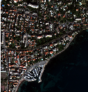
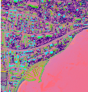
Figure 18.1: Result of applying the otb::PCAImageFilter to an image. From left to right: original image, color composition with first three principal components and output of the inverse mode (the input RGB image).


18.2 Noise-Adjusted Principal Components Analysis

The source code for this example can be found in the file
Examples/DimensionReduction/NAPCAExample.cxx.

This example illustrates the use of the otb::NAPCAImageFilter . This filter computes a Noise-Adjusted Principal Component Analysis transform [86] using an efficient method based on the inner product in order to compute the covariance matrix.

The Noise-Adjusted Principal Component Analysis transform is a sequence of two Principal Component Analysis transforms. The first transform is based on an estimated covariance matrix of the noise, and intends to whiten the input image (noise with unit variance and no correlation between bands).

The second Principal Component Analysis is then applied to the noise-whitened image, giving the Maximum Noise Fraction transform. Applying PCA on noise-whitened image consists in ranking Principal Components according to signal to noise ratio.

It is basically a reformulation of the Maximum Noise Fraction algorithm.

The first step required to use this filter is to include its header file.

  #include "otbNAPCAImageFilter.h"

We also need to include the header of the noise filter.

  #include "otbLocalActivityVectorImageFilter.h"

We start by defining the types for the images, the reader and the writer. We choose to work with a otb::VectorImage , since we will produce a multi-channel image (the principal components) from a multi-channel input image.

    typedef otb::VectorImage<PixelType, Dimension> ImageType;
    typedef otb::ImageFileReader<ImageType>        ReaderType;
    typedef otb::ImageFileWriter<ImageType>        WriterType;

We instantiate now the image reader and we set the image file name.

    ReaderType::Pointer reader     = ReaderType::New();
    reader->SetFileName(inputFileName);

In contrast with standard Principal Component Analysis, NA-PCA needs an estimation of the noise correlation matrix in the dataset prior to transformation.

A classical approach is to use spatial gradient images and infer the noise correlation matrix from it. The method of noise estimation can be customized by templating the otb::NAPCAImageFilter with the desired noise estimation method.

In this implementation, noise is estimated from a local window. We define the type of the noise filter.

    typedef otb::LocalActivityVectorImageFilter<ImageType,ImageType> NoiseFilterType;

We define the type for the filter. It is templated over the input and the output image types, the noise estimation filter type, and also the transformation direction. The internal structure of this filter is a filter-to-filter like structure. We can now the instantiate the filter.

    typedef otb::NAPCAImageFilter<ImageType, ImageType,
                                  NoiseFilterType,
                                  otb::Transform::FORWARD> NAPCAFilterType;
    NAPCAFilterType::Pointer napcafilter     = NAPCAFilterType::New();

We then set the number of principal components required as output. We can choose to get less PCs than the number of input bands.

    napcafilter->SetNumberOfPrincipalComponentsRequired(
      numberOfPrincipalComponentsRequired);

We set the radius of the sliding window for noise estimation.

    NoiseFilterType::RadiusType radius = {{ vradius, vradius }};
    napcafilter->GetNoiseImageFilter()->SetRadius(radius);

Last, we can activate normalisation.

    napcafilter->SetUseNormalization( normalization );

We now instantiate the writer and set the file name for the output image.

    WriterType::Pointer writer     = WriterType::New();
    writer->SetFileName(outputFilename);

We finally plug the pipeline and trigger the NA-PCA computation with the method Update() of the writer.

    napcafilter->SetInput(reader->GetOutput());
    writer->SetInput(napcafilter->GetOutput());
  
    writer->Update();

otb::NAPCAImageFilter allows also to compute inverse transformation from NA-PCA coefficients. In reverse mode, the covariance matrix or the transformation matrix (which may not be square) has to be given.

    typedef otb::NAPCAImageFilter< ImageType, ImageType,
                                   NoiseFilterType,
                                   otb::Transform::INVERSE > InvNAPCAFilterType;
    InvNAPCAFilterType::Pointer invFilter = InvNAPCAFilterType::New();
  
    invFilter->SetMeanValues( napcafilter->GetMeanValues() );
    if ( normalization )
      invFilter->SetStdDevValues( napcafilter->GetStdDevValues() );
    invFilter->SetTransformationMatrix( napcafilter->GetTransformationMatrix() );
    invFilter->SetInput(napcafilter->GetOutput());
  
    WriterType::Pointer invWriter = WriterType::New();
    invWriter->SetFileName(outputInverseFilename );
    invWriter->SetInput(invFilter->GetOutput() );
  
    invWriter->Update();

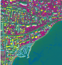
Figure 18.2 shows the result of applying forward and reverse NA-PCA transformation to a 8 bands Worldview2 image.


PIC PIC PIC

Figure 18.2: Result of applying the otb::NAPCAImageFilter to an image. From left to right: original image, color composition with first three principal components and output of the inverse mode (the input RGB image).


18.3 Maximum Noise Fraction

The source code for this example can be found in the file
Examples/DimensionReduction/MNFExample.cxx.

This example illustrates the use of the otb::MNFImageFilter . This filter computes a Maximum Noise Fraction transform [52] using an efficient method based on the inner product in order to compute the covariance matrix.

The Maximum Noise Fraction transform is a sequence of two Principal Component Analysis transforms. The first transform is based on an estimated covariance matrix of the noise, and intends to whiten the input image (noise with unit variance and no correlation between bands).

The second Principal Component Analysis is then applied to the noise-whitened image, giving the Maximum Noise Fraction transform.

In this implementation, noise is estimated from a local window.

The first step required to use this filter is to include its header file.

  #include "otbMNFImageFilter.h"

We also need to include the header of the noise filter.

  #include "otbLocalActivityVectorImageFilter.h"

We start by defining the types for the images, the reader, and the writer. We choose to work with a otb::VectorImage , since we will produce a multi-channel image (the principal components) from a multi-channel input image.

    typedef otb::VectorImage<PixelType, Dimension> ImageType;
    typedef otb::ImageFileReader<ImageType>        ReaderType;
    typedef otb::ImageFileWriter<ImageType>        WriterType;

We instantiate now the image reader and we set the image file name.

    ReaderType::Pointer reader     = ReaderType::New();
    reader->SetFileName(inputFileName);

In contrast with standard Principal Component Analysis, MNF needs an estimation of the noise correlation matrix in the dataset prior to transformation.

A classical approach is to use spatial gradient images and infer the noise correlation matrix from it. The method of noise estimation can be customized by templating the otb::MNFImageFilter with the desired noise estimation method.

In this implementation, noise is estimated from a local window. We define the type of the noise filter.

    typedef otb::LocalActivityVectorImageFilter<ImageType,ImageType> NoiseFilterType;

We define the type for the filter. It is templated over the input and the output image types and also the transformation direction. The internal structure of this filter is a filter-to-filter like structure. We can now the instantiate the filter.

    typedef otb::MNFImageFilter<ImageType, ImageType,
                                  NoiseFilterType,
                                  otb::Transform::FORWARD> MNFFilterType;
    MNFFilterType::Pointer MNFfilter     = MNFFilterType::New();

We then set the number of principal components required as output. We can choose to get less PCs than the number of input bands.

    MNFfilter->SetNumberOfPrincipalComponentsRequired(
      numberOfPrincipalComponentsRequired);

We set the radius of the sliding window for noise estimation.

    NoiseFilterType::RadiusType radius = {{ vradius, vradius }};
    MNFfilter->GetNoiseImageFilter()->SetRadius(radius);

Last, we can activate normalisation.

    MNFfilter->SetUseNormalization( normalization );

We now instantiate the writer and set the file name for the output image.

    WriterType::Pointer writer     = WriterType::New();
    writer->SetFileName(outputFilename);

We finally plug the pipeline and trigger the MNF computation with the method Update() of the writer.

    MNFfilter->SetInput(reader->GetOutput());
    writer->SetInput(MNFfilter->GetOutput());
  
    writer->Update();

otb::MNFImageFilter allows also to compute inverse transformation from MNF coefficients. In reverse mode, the covariance matrix or the transformation matrix (which may not be square) has to be given.

    typedef otb::MNFImageFilter< ImageType, ImageType,
                                   NoiseFilterType,
                                   otb::Transform::INVERSE > InvMNFFilterType;
    InvMNFFilterType::Pointer invFilter = InvMNFFilterType::New();
  
    invFilter->SetMeanValues( MNFfilter->GetMeanValues() );
    if ( normalization )
      invFilter->SetStdDevValues( MNFfilter->GetStdDevValues() );
    invFilter->SetTransformationMatrix( MNFfilter->GetTransformationMatrix() );
    invFilter->SetInput(MNFfilter->GetOutput());
  
    WriterType::Pointer invWriter = WriterType::New();
    invWriter->SetFileName(outputInverseFilename );
    invWriter->SetInput(invFilter->GetOutput() );
  
    invWriter->Update();

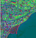
Figure 18.3 shows the result of applying forward and reverse MNF transformation to a 8 bands Worldview2 image.


PIC PIC PIC

Figure 18.3: Result of applying the otb::MNFImageFilter to an image. From left to right: original image, color composition with first three principal components and output of the inverse mode (the input RGB image).


18.4 Fast Independent Component Analysis

The source code for this example can be found in the file
Examples/DimensionReduction/ICAExample.cxx.

This example illustrates the use of the otb::FastICAImageFilter . This filter computes a Fast Independent Components Analysis transform.

Like Principal Components Analysis, Independent Component Analysis [77] computes a set of orthogonal linear combinations, but the criterion of Fast ICA is different: instead of maximizing variance, it tries to maximize statistical independence between components.

In the Fast ICA algorithm [66], statistical independence is measured by evaluating non-Gaussianity of the components, and the maximization is done in an iterative way.

The first step required to use this filter is to include its header file.

  #include "otbFastICAImageFilter.h"

We start by defining the types for the images, the reader, and the writer. We choose to work with a otb::VectorImage , since we will produce a multi-channel image (the independent components) from a multi-channel input image.

    typedef otb::VectorImage<PixelType, Dimension> ImageType;
    typedef otb::ImageFileReader<ImageType>        ReaderType;
    typedef otb::ImageFileWriter<ImageType>        WriterType;

We instantiate now the image reader and we set the image file name.

    ReaderType::Pointer reader     = ReaderType::New();
    reader->SetFileName(inputFileName);

We define the type for the filter. It is templated over the input and the output image types and also the transformation direction. The internal structure of this filter is a filter-to-filter like structure. We can now the instantiate the filter.

    typedef otb::FastICAImageFilter<ImageType, ImageType,
                                  otb::Transform::FORWARD> FastICAFilterType;
    FastICAFilterType::Pointer FastICAfilter     = FastICAFilterType::New();

We then set the number of independent components required as output. We can choose to get less ICs than the number of input bands.

    FastICAfilter->SetNumberOfPrincipalComponentsRequired(
      numberOfPrincipalComponentsRequired);

We set the number of iterations of the ICA algorithm.

    FastICAfilter->SetNumberOfIterations(numIterations);

We also set the μ parameter.

    FastICAfilter->SetMu( mu );

We now instantiate the writer and set the file name for the output image.

    WriterType::Pointer writer     = WriterType::New();
    writer->SetFileName(outputFilename);

We finally plug the pipeline and trigger the ICA computation with the method Update() of the writer.

    FastICAfilter->SetInput(reader->GetOutput());
    writer->SetInput(FastICAfilter->GetOutput());
  
    writer->Update();

otb::FastICAImageFilter allows also to compute inverse transformation from ICA coefficients. In reverse mode, the covariance matrix or the transformation matrix (which may not be square) has to be given.

    typedef otb::FastICAImageFilter< ImageType, ImageType,
                                   otb::Transform::INVERSE > InvFastICAFilterType;
    InvFastICAFilterType::Pointer invFilter = InvFastICAFilterType::New();
  
    invFilter->SetMeanValues( FastICAfilter->GetMeanValues() );
    invFilter->SetStdDevValues( FastICAfilter->GetStdDevValues() );
    invFilter->SetTransformationMatrix( FastICAfilter->GetTransformationMatrix() );
    invFilter->SetPCATransformationMatrix(
                              FastICAfilter->GetPCATransformationMatrix() );
    invFilter->SetInput(FastICAfilter->GetOutput());
  
    WriterType::Pointer invWriter = WriterType::New();
    invWriter->SetFileName(outputInverseFilename );
    invWriter->SetInput(invFilter->GetOutput() );
  
    invWriter->Update();

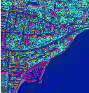
Figure 18.4 shows the result of applying forward and reverse FastICA transformation to a 8 bands Worldview2 image.


PIC PIC PIC

Figure 18.4: Result of applying the otb::FastICAImageFilter to an image. From left to right: original image, color composition with first three independent components and output of the inverse mode (the input RGB image).


18.5 Maximum Autocorrelation Factor

The source code for this example can be found in the file
Examples/DimensionReduction/MaximumAutocorrelationFactor.cxx.

This example illustrates the class otb::MaximumAutocorrelationFactorImageFilter , which performs a Maximum Autocorrelation Factor transform [100]. Like PCA, MAF tries to find a set of orthogonal linear transform, but the criterion to maximize is the spatial auto-correlation rather than the variance.

Auto-correlation is the correlation between the component and a unitary shifted version of the component.

Please note that the inverse transform is not implemented yet.

We start by including the corresponding header file.

  #include "otbMaximumAutocorrelationFactorImageFilter.h"

We then define the types for the input image and the output image.

    typedef otb::VectorImage<unsigned short, 2> InputImageType;
    typedef otb::VectorImage<double, 2>         OutputImageType;

We can now declare the types for the reader. Since the images can be very large, we will force the pipeline to use streaming. For this purpose, the file writer will be streamed. This is achieved by using the otb::ImageFileWriter class.

    typedef otb::ImageFileReader<InputImageType>    ReaderType;
    typedef otb::ImageFileWriter<OutputImageType> WriterType;

The otb::MultivariateAlterationDetectorImageFilter is templated over the type of the input images and the type of the generated change image.

    typedef otb::MaximumAutocorrelationFactorImageFilter<InputImageType,
                                            OutputImageType> FilterType;

The different elements of the pipeline can now be instantiated.

    ReaderType::Pointer reader = ReaderType::New();
    WriterType::Pointer writer = WriterType::New();
    FilterType::Pointer filter = FilterType::New();

We set the parameters of the different elements of the pipeline.

    reader->SetFileName(infname);
    writer->SetFileName(outfname);

We build the pipeline by plugging all the elements together.

    filter->SetInput(reader->GetOutput());
    writer->SetInput(filter->GetOutput());

And then we can trigger the pipeline update, as usual.

    writer->Update();

Figure 18.5 shows the results of Maximum Autocorrelation Factor applied to an 8 bands Worldview2 image.


PIC PIC

Figure 18.5: Results of the Maximum Autocorrelation Factor algorithm applied to a 8 bands Worldview2 image (3 first components).