Chapter 13
Image Fusion

Satellite sensors present an important diversity in terms of characteristics. Some provide a high spatial resolution while other focus on providing several spectral bands. The fusion process brings the information from different sensors with different characteristics together to get the best of both worlds.

Most of the fusion methods in the remote sensing community deal with the pansharpening technique. This fusion combines the image from the PANchromatic sensor of one satellite (high spatial resolution data) with the multispectral (XS) data (lower resolution in several spectral bands) to generate images with a high resolution and several spectral bands. Several advantages make this situation easier:

• PAN and XS images are taken simultaneously from the same satellite (or with a very short delay);
• the imaged area is common to both scenes;
• many satellites provide these data (SPOT 1-5, Quickbird, Pleiades)

This case is well-studied in the literature and many methods exist. Only very few are available in OTB now but this should evolve soon.

13.1 Simple Pan Sharpening

A simple way to view the pan-sharpening of data is to consider that, at the same resolution, the panchromatic channel is the sum of the XS channel. After putting the two images in the same geometry, after orthorectification (see chapter 11) with an oversampling of the XS image, we can proceed to the data fusion.

The idea is to apply a low pass filter to the panchromatic band to give it a spectral content (in the Fourier domain) equivalent to the XS data. Then we normalize the XS data with this low-pass panchromatic and multiply the result with the original panchromatic band.

The process is described on figure 13.1.

The source code for this example can be found in the file
Examples/Fusion/PanSharpeningExample.cxx.

Here we are illustrating the use of the otb::SimpleRcsPanSharpeningFusionImageFilter for PAN-sharpening. This example takes a PAN and the corresponding XS images as input. These images are supposed to be registered.

The fusion operation is defined as

(13.1)

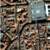
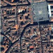
Figure 13.2 shows the result of applying this PAN sharpening filter to a Quickbird image.

We start by including the required header and declaring the main function:

We declare the different image type used here as well as the image reader. Note that, the reader for the PAN image is templated by an otb::Image while the XS reader uses an otb::VectorImage .

We pass the filenames to the readers

We declare the fusion filter an set its inputs using the readers:

And finally, we declare the writer and call its Update() method to trigger the full pipeline execution.

13.2 Bayesian Data Fusion

The source code for this example can be found in the file
Examples/Fusion/BayesianFusionImageFilter.cxx.

The following example illustrates the use of the otb::BayesianFusionFilter . The Bayesian data fusion relies on the idea that variables of interest, denoted as vector Z, cannot be directly observed. They are linked to the observable variables Y through the following error-like model.

(13.2)

where g(Z) is a set of functionals and E is a vector of random errors that are stochastically independent from Z. This algorithm uses elementary probability calculus, and several assumptions to compute the data fusion. For more explication see Fasbender, Radoux and Bogaert’s publication [41]. Three images are used :

• a panchromatic image,
• a multispectral image resampled at the panchromatic image spatial resolution,
• a multispectral image resampled at the panchromatic image spatial resolution, using, e.g. a cubic interpolator.
• a float : λ, the meaning of the weight to be given to the panchromatic image compared to the multispectral one.

Let’s look at the minimal code required to use this algorithm. First, the following header defining the otb::BayesianFusionFilter class must be included.

The image types are now defined using pixel types and particular dimension. The panchromatic image is defined as an otb::Image and the multispectral one as otb::VectorImage .

The Bayesian data fusion filter type is instantiated using the images types as a template parameters.

Next the filter is created by invoking the New() method and assigning the result to a itk::SmartPointer .

Now the multi spectral image, the interpolated multi spectral image and the panchromatic image are given as inputs to the filter.

The BayesianFusionFilter requires defining one parameter : λ. The λ parameter can be used to tune the fusion toward either a high color consistency or sharp details. Typical λ value range in [0.5,1[, where higher values yield sharper details. by default λ is set at 0.9999.

The invocation of the Update() method on the writer triggers the execution of the pipeline. It is recommended to place update calls in a try/catch block in case errors occur and exceptions are thrown.

Let’s now run this example using as input the images multiSpect.tif , multiSpectInterp.tif and panchro.tif provided in the directory Examples/Data. The results obtained for 2 different values for λ are shown in figure 13.3.