Change detection techniques try to detect and locate areas which have changed between two or more
observations of the same scene. These changes can be of different types, with different origins and of
different temporal length. This allows to distinguish different kinds of applications:
- land use monitoring, which corresponds to the characterization of the evolution of the
vegetation, or its seasonal changes;
- natural resources management, which corresponds mainly to the characterization of the
evolution of the urban areas, the evolution of the deforestation, etc.
- damage mapping, which corresponds to the location of damages caused by natural or
industrial disasters.
From the point of view of the observed phenomena, one can distinguish 2 types of changes whose nature is
rather different: the abrupt changes and the progressive changes, which can eventually be periodic. From the
data point of view, one can have:
- Image pairs before and after the event. The applications are mainly the abrupt changes.
- Multi-temporal image series on which 2 types on changes may appear:
- The slow changes like for instance the erosion, vegetation evolution, etc. The
knowledge of the studied phenomena and of their consequences on the geometrical and
radiometrical evolution at the different dates is a very important information for this kind
of analysis.
- The abrupt changes may pose different kinds of problems depending on whether the date
of the change is known in the image series or not. The detection of areas affected by a
change occurred at a known date may exploit this a priori information in order to split
the image series into two sub-series (before an after) and use the temporal redundancy
in order to improve the detection results. On the other hand, when the date of the change
is not known, the problem has a higher difficulty.
From this classification of the different types of problems, one can infer 4 cases for which one can look for
algorithms as a function of the available data:
- Abrupt changes in an image pair. This is no doubt the field for which more work has been
done. One can find tools at the 3 classical levels of image processing: data level (differences,
ratios, with or without pre-filtering, etc.), feature level (edges, targets, etc.), and interpretation
level (post-classification comparison).
- Abrupt changes within an image series and a known date. One can rely on bi-date techniques,
either by fusing the images into 2 stacks (before and after), or by fusing the results obtained
by different image couples (one after and one before the event). One can also use specific
discontinuity detection techniques to be applied in the temporal axis.
- Abrupt changes within an image series and an unknown date. This case can be seen either as
a generalization of the preceding one (testing the N-1 positions for N dates) or as a particular
case of the following one.
- Progressive changes within an image series. One can work in two steps:
- detect the change areas using stability criteria in the temporal areas;
- identify the changes using prior information about the type of changes of interest.
In this section we discuss about the damage assessment techniques which can be applied when only two
images (before/after) are available.
As it has been shown in recent review works [30, 90, 113, 115], a relatively high number of methods exist,
but most of them have been developed for optical and infrared sensors. Only a few recent works on change
detection with radar images exist [126, 16, 101, 69, 38, 11, 71]. However, the intrinsic limits of passive
sensors, mainly related to their dependence on meteorological and illumination conditions, impose severe
constraints for operational applications. The principal difficulties related to change detection are of four
types:
- In the case of radar images, the speckle noise makes the image exploitation difficult.
- The geometric configuration of the image acquisition can produce images which are difficult
to compare.
- Also, the temporal gap between the two acquisitions and thus the sensor aging and the
inter-calibration are sources of variability which are difficult to deal with.
- Finally, the normal evolution of the observed scenes must not be confused with the changes
of interest.
The problem of detecting abrupt changes between a pair of images is the following: Let I1,I2 be two images
acquired at different dates t1,t2; we aim at producing a thematic map which shows the areas where changes
have taken place.
Three main categories of methods exist:
- Strategy 1: Post Classification Comparison
The principle of this approach [34] is two obtain two land-use maps independently for each
date and comparing them.
- Strategy 2: Joint classification
This method consists in producing the change map directly from a joint classification of both
images.
- Strategy 3: Simple detectors
The last approach consists in producing an image of change likelihood (by differences, ratios
or any other approach) and thresholding it in order to produce the change map.
Because of its simplicity and its low computation overhead, the third strategy is the one which has been
chosen for the processing presented here.
The source code for this example can be found in the file
Examples/ChangeDetection/ChangeDetectionFrameworkExample.cxx.
This example illustrates the Change Detector framework implemented in OTB. This framework uses the generic
programming approach. All change detection filters are otb::BinaryFunctorNeighborhoodImageFilter s,
that is, they are filters taking two images as input and provide one image as output. The change detection
computation itself is performed on the neighborhood of each pixel of the input images.
The first step in building a change detection filter is to include the header of the parent class.
#include "otbBinaryFunctorNeighborhoodImageFilter.h"
The change detection operation itself is one of the templates of the change detection filters and takes the
form of a function, that is, something accepting the syntax foo(). This can be implemented using classical
C/C++ functions, but it is preferable to implement it using C++ functors. These are classical C++
classes which overload the () operator. This allows to be used with the same syntax as C/C++
functions.
Since change detectors operate on neighborhoods, the functor call will take 2 arguments which are
itk::ConstNeighborhoodIterator s.
The change detector functor is templated over the types of the input iterators and the output result type. The
core of the change detection is implemented in the operator() section.
template<class TInput1, class TInput2, class TOutput> class MyChangeDetector { public:
// The constructor and destructor. MyChangeDetector() {} ~MyChangeDetector() {}
// Change detection operation inline TOutput operator ()(const TInput1& itA,
const TInput2& itB) { TOutput result = 0.0;
for (unsigned long pos = 0; pos < itA.Size(); ++pos) {
result += static_cast<TOutput>(itA.GetPixel(pos) - itB.GetPixel(pos)); }
return static_cast<TOutput>(result / itA.Size()); } };
The interest of using functors is that complex operations can be performed using internal protected class
methods and that class variables can be used to store information so different pixel locations can access to
results of previous computations.
The next step is the definition of the change detector filter. As stated above, this filter will inherit from
otb::BinaryFunctorNeighborhoodImageFilter which is templated over the 2 input image types, the
output image type and the functor used to perform the change detection operation.
Inside the class only a few typedefs and the constructors and destructors need to be declared.
template <class TInputImage1, class TInputImage2, class TOutputImage>
class ITK_EXPORT MyChangeDetectorImageFilter : public otb::BinaryFunctorNeighborhoodImageFilter<
TInputImage1, TInputImage2, TOutputImage, MyChangeDetector<
typename itk::ConstNeighborhoodIterator<TInputImage1>,
typename itk::ConstNeighborhoodIterator<TInputImage2>, typename TOutputImage::PixelType> >
{ public: /⋆⋆ Standard class typedefs. ⋆/ typedef MyChangeDetectorImageFilter Self;
typedef typename otb::BinaryFunctorNeighborhoodImageFilter< TInputImage1, TInputImage2, TOutputImage,
MyChangeDetector< typename itk::ConstNeighborhoodIterator<TInputImage1>,
typename itk::ConstNeighborhoodIterator<TInputImage2>,
typename TOutputImage::PixelType> > Superclass;
typedef itk::SmartPointer<Self> Pointer; typedef itk::SmartPointer<const Self> ConstPointer;
/⋆⋆ Method for creation through the object factory. ⋆/ itkNewMacro(Self);
protected: MyChangeDetectorImageFilter() {} ~MyChangeDetectorImageFilter() ITK_OVERRIDE {}
private: MyChangeDetectorImageFilter(const Self &); //purposely not implemented
void operator =(const Self&); //purposely not implemented };
Pay particular attention to the fact that no .txx file is needed, since the filtering operation is implemented in
the otb::BinaryFunctorNeighborhoodImageFilter class. So all the algorithmics part is inside the
functor.
We can now write a program using the change detector.
As usual, we start by defining the image types. The internal computations will be performed using floating
point precision, while the output image will be stored using one byte per pixel.
typedef float InternalPixelType;
typedef unsigned char OutputPixelType;
typedef otb::Image<InternalPixelType, Dimension> InputImageType1;
typedef otb::Image<InternalPixelType, Dimension> InputImageType2;
typedef otb::Image<InternalPixelType, Dimension> ChangeImageType;
typedef otb::Image<OutputPixelType, Dimension> OutputImageType;
We declare the readers, the writer, but also the itk::RescaleIntensityImageFilter which will be
used to rescale the result before writing it to a file.
typedef otb::ImageFileReader<InputImageType1> ReaderType1;
typedef otb::ImageFileReader<InputImageType2> ReaderType2;
typedef otb::ImageFileWriter<OutputImageType> WriterType;
typedef itk::RescaleIntensityImageFilter<ChangeImageType, OutputImageType> RescalerType;
The next step is to declare the filter for the change detection.
typedef MyChangeDetectorImageFilter<InputImageType1, InputImageType2, ChangeImageType> FilterType;
We connect the pipeline.
reader1->SetFileName(inputFilename1); reader2->SetFileName(inputFilename2);
writer->SetFileName(outputFilename); rescaler->SetOutputMinimum(itk::NumericTraits<OutputPixelType>::min());
rescaler->SetOutputMaximum(itk::NumericTraits<OutputPixelType>::max()); filter->SetInput1(reader1->GetOutput());
filter->SetInput2(reader2->GetOutput()); filter->SetRadius(atoi(argv[3]));
rescaler->SetInput(filter->GetOutput()); writer->SetInput(rescaler->GetOutput());
And that is all.
The simplest change detector is based on the pixel-wise differencing of image values:
 | (21.1) |
In order to make the algorithm robust to noise, one actually uses local means instead of pixel
values.
The source code for this example can be found in the file
Examples/ChangeDetection/DiffChDet.cxx.
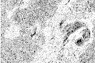
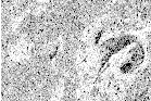
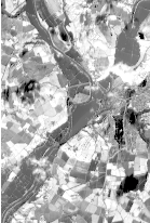
This example illustrates the class otb::MeanDifferenceImageFilter for detecting changes between
pairs of images. This filter computes the mean intensity in the neighborhood of each pixel of the pair of
images to be compared and uses the difference of means as a change indicator. This example will use the
images shown in figure 21.1. These correspond to the near infrared band of two Spot acquisitions before
and during a flood.
We start by including the corresponding header file.
#include "otbMeanDifferenceImageFilter.h"
We start by declaring the types for the two input images, the change image and the image to be stored in a
file for visualization.
typedef float InternalPixelType;
typedef unsigned char OutputPixelType;
typedef otb::Image<InternalPixelType, Dimension> InputImageType1;
typedef otb::Image<InternalPixelType, Dimension> InputImageType2;
typedef otb::Image<InternalPixelType, Dimension> ChangeImageType;
typedef otb::Image<OutputPixelType, Dimension> OutputImageType;
We can now declare the types for the readers and the writer.
typedef otb::ImageFileReader<InputImageType1> ReaderType1;
typedef otb::ImageFileReader<InputImageType2> ReaderType2;
typedef otb::ImageFileWriter<OutputImageType> WriterType;
The change detector will give positive and negative values depending on the sign of the difference. We are
usually interested only in the absolute value of the difference. For this purpose, we will use the
itk::AbsImageFilter . Also, before saving the image to a file in, for instance, PNG format, we will
rescale the results of the change detection in order to use the full range of values of the output pixel
type.
typedef itk::AbsImageFilter<ChangeImageType, ChangeImageType> AbsType;
typedef itk::RescaleIntensityImageFilter<ChangeImageType, OutputImageType> RescalerType;
The otb::MeanDifferenceImageFilter is templated over the types of the two input images and the
type of the generated change image.
typedef otb::MeanDifferenceImageFilter< InputImageType1, InputImageType2,
ChangeImageType> FilterType;
The different elements of the pipeline can now be instantiated.
ReaderType1::Pointer reader1 = ReaderType1::New(); ReaderType2::Pointer reader2 = ReaderType2::New();
WriterType::Pointer writer = WriterType::New(); FilterType::Pointer filter = FilterType::New();
AbsType::Pointer absFilter = AbsType::New(); RescalerType::Pointer rescaler = RescalerType::New();
We set the parameters of the different elements of the pipeline.
reader1->SetFileName(inputFilename1); reader2->SetFileName(inputFilename2);
writer->SetFileName(outputFilename); rescaler->SetOutputMinimum(itk::NumericTraits<OutputPixelType>::min());
rescaler->SetOutputMaximum(itk::NumericTraits<OutputPixelType>::max());
The only parameter for this change detector is the radius of the window used for computing the mean of the
intensities.
filter->SetRadius(atoi(argv[4]));
We build the pipeline by plugging all the elements together.
filter->SetInput1(reader1->GetOutput()); filter->SetInput2(reader2->GetOutput());
absFilter->SetInput(filter->GetOutput()); rescaler->SetInput(absFilter->GetOutput());
writer->SetInput(rescaler->GetOutput());
Since the processing time of large images can be long, it is interesting to monitor the evolution of the
computation. In order to do so, the change detectors can use the command/observer design pattern. This is
easily done by attaching an observer to the filter.
typedef otb::CommandProgressUpdate<FilterType> CommandType;
CommandType::Pointer observer = CommandType::New(); filter->AddObserver(itk::ProgressEvent(), observer);
Figure 21.2 shows the result of the change detection by difference of local means.
This detector is similar to the previous one except that it uses a ratio instead of the difference:
 | (21.2) |
The use of the ratio makes this detector robust to multiplicative noise which is a good model for the speckle
phenomenon which is present in radar images.
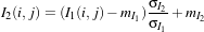
In order to have a bounded and normalized detector the following expression is actually used:
 | (21.3) |
The source code for this example can be found in the file
Examples/ChangeDetection/RatioChDet.cxx.
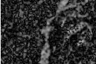
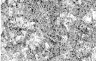
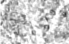
This example illustrates the class otb::MeanRatioImageFilter for detecting changes between pairs of
images. This filter computes the mean intensity in the neighborhood of each pixel of the pair of images to
be compared and uses the ratio of means as a change indicator. This change indicator is then normalized
between 0 and 1 by using the classical
 | (21.4) |
where μA and μB are the local means. This example will use the images shown in figure 21.3. These
correspond to 2 Radarsat fine mode acquisitions before and after a lava flow resulting from a volcanic
eruption.
We start by including the corresponding header file.
#include "otbMeanRatioImageFilter.h"
We start by declaring the types for the two input images, the change image and the image to be stored in a
file for visualization.
typedef float InternalPixelType;
typedef unsigned char OutputPixelType;
typedef otb::Image<InternalPixelType, Dimension> InputImageType1;
typedef otb::Image<InternalPixelType, Dimension> InputImageType2;
typedef otb::Image<InternalPixelType, Dimension> ChangeImageType;
typedef otb::Image<OutputPixelType, Dimension> OutputImageType;
We can now declare the types for the readers. Since the images can be vey large, we will force the pipeline
to use streaming. For this purpose, the file writer will be streamed. This is achieved by using the
otb::ImageFileWriter class.
typedef otb::ImageFileReader<InputImageType1> ReaderType1;
typedef otb::ImageFileReader<InputImageType2> ReaderType2;
typedef otb::ImageFileWriter<OutputImageType> WriterType;
The change detector will give a normalized result between 0 and 1. In order to store the result in PNG
format we will rescale the results of the change detection in order to use all the output pixel type range of
values.
typedef itk::ShiftScaleImageFilter<ChangeImageType, OutputImageType> RescalerType;
The otb::MeanRatioImageFilter is templated over the types of the two input images and the type of
the generated change image.
typedef otb::MeanRatioImageFilter< InputImageType1, InputImageType2,
ChangeImageType> FilterType;
The different elements of the pipeline can now be instantiated.
ReaderType1::Pointer reader1 = ReaderType1::New(); ReaderType2::Pointer reader2 = ReaderType2::New();
WriterType::Pointer writer = WriterType::New(); FilterType::Pointer filter = FilterType::New();
RescalerType::Pointer rescaler = RescalerType::New();
We set the parameters of the different elements of the pipeline.
reader1->SetFileName(inputFilename1); reader2->SetFileName(inputFilename2);
writer->SetFileName(outputFilename); float scale = itk::NumericTraits<OutputPixelType>::max();
rescaler->SetScale(scale);
The only parameter for this change detector is the radius of the window used for computing the mean of the
intensities.
filter->SetRadius(atoi(argv[4]));
We build the pipeline by plugging all the elements together.
filter->SetInput1(reader1->GetOutput()); filter->SetInput2(reader2->GetOutput());
rescaler->SetInput(filter->GetOutput()); writer->SetInput(rescaler->GetOutput());
Figure 21.4 shows the result of the change detection by ratio of local means.
This detector is similar to the ratio of means detector (seen in the previous section page 922). Nevertheless,
instead of the comparison of means, the comparison is performed to the complete distribution of the two
Random Variables (RVs) [69].
The detector is based on the Kullback-Leibler distance between probability density functions (pdfs). In the
neighborhood of each pixel of the pair of images I1 and I2 to be compared, the distance between local pdfs
f1 and f2 of RVs X1 and X2 is evaluated by:
 (X1,X2) (X1,X2) | = K(X1|X2)+K(X2|X1) | (21.5)
|
| with K(Xj|Xi) | = ∫
Rlog fXi(x)dx, i,j = 1,2. fXi(x)dx, i,j = 1,2. | (21.6) |
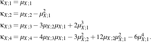
In order to reduce the computational time, the local pdfs f1 and f2 are not estimated through histogram
computations but rather by a cumulant expansion, namely the Edgeworth expansion, with is based on the
cumulants of the RVs:
 | (21.7) |
In eq. (21.7),  X stands for the Gaussian pdf which has the same mean and variance as the RV X. The κX;k
coefficients are the cumulants of order k, and Hk(x) are the Chebyshev-Hermite polynomials of order k
(see [71] for deeper explanations).
X stands for the Gaussian pdf which has the same mean and variance as the RV X. The κX;k
coefficients are the cumulants of order k, and Hk(x) are the Chebyshev-Hermite polynomials of order k
(see [71] for deeper explanations).
The source code for this example can be found in the file
Examples/ChangeDetection/KullbackLeiblerDistanceChDet.cxx.
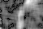
This example illustrates the class otb::KullbackLeiblerDistanceImageFilter for detecting changes
between pairs of images. This filter computes the Kullback-Leibler distance between probability density
functions (pdfs). In fact, the Kullback-Leibler distance is itself approximated through a cumulant-based
expansion, since the pdfs are approximated through an Edgeworth series. The Kullback-Leibler distance is
evaluated by:
 |
(21.8)
|
where
| a1 | = c3 -3 a2 a2 | = c4 -6 + + a3 a3 | = c6 -15 +45 +45 - - c2 c2 | = α2 +β2c3 | = α3 +3αβ2c4 | = α4 +6α2β2 +3β4c
6 | = α6 +15α4β2 +45α2β4 +15β6α | =  β β | =  . . | | | | | | | | | | |
κXi;1, κXi;2, κXi;3 and κXi;4 are the cumulants up to order 4 of the random variable Xi (i = 1,2). This
example will use the images shown in figure 21.3. These correspond to 2 Radarsat fine mode acquisitions
before and after a lava flow resulting from a volcanic eruption.
The program itself is very similar to the ratio of means detector, implemented in otb::MeanRatioImageFilter
, in section 21.3.2. Nevertheless the corresponding header file has to be used instead.
#include "otbKullbackLeiblerDistanceImageFilter.h"
The otb::KullbackLeiblerDistanceImageFilter is templated over the types of the two input images
and the type of the generated change image, in a similar way as the otb::MeanRatioImageFilter . It is
the only line to be changed from the ratio of means change detection example to perform a change detection
through a distance between distributions...
typedef otb::KullbackLeiblerDistanceImageFilter<ImageType, ImageType, ImageType> FilterType;
The different elements of the pipeline can now be instantiated. Follow the ratio of means change detector
example.
The only parameter for this change detector is the radius of the window used for computing the
cumulants.
FilterType::Pointer filter = FilterType::New(); filter->SetRadius((winSize - 1) / 2);
The pipeline is built by plugging all the elements together.
filter->SetInput1(reader1->GetOutput()); filter->SetInput2(reader2->GetOutput());
Figure 21.5 shows the result of the change detection by computing the Kullback-Leibler distance
between local pdf through an Edgeworth approximation.
The correlation coefficient measures the likelihood of a linear relationship between two random
variables:
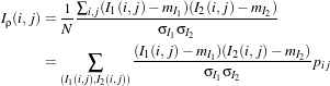 | (21.9) |
where I1(i,j) and I2(i,j) are the pixel values of the 2 images and pij is the joint probability density. This is
like using a linear model:
 | (21.10) |
for which we evaluate the likelihood with pij.
With respect to the difference detector, this one will be robust to illumination changes.
The source code for this example can be found in the file
Examples/ChangeDetection/CorrelChDet.cxx.
This example illustrates the class otb::CorrelationChangeDetector for detecting changes between
pairs of images. This filter computes the correlation coefficient in the neighborhood of each pixel of the pair
of images to be compared. This example will use the images shown in figure 21.6. These correspond to
two ERS acquisitions before and during a flood.
We start by including the corresponding header file.
#include "otbCorrelationChangeDetector.h"
We start by declaring the types for the two input images, the change image and the image to be stored in a
file for visualization.
typedef float InternalPixelType;
typedef unsigned char OutputPixelType;
typedef otb::Image<InternalPixelType, Dimension> InputImageType1;
typedef otb::Image<InternalPixelType, Dimension> InputImageType2;
typedef otb::Image<InternalPixelType, Dimension> ChangeImageType;
typedef otb::Image<OutputPixelType, Dimension> OutputImageType;
We can now declare the types for the readers. Since the images can be vey large, we will force the pipeline
to use streaming. For this purpose, the file writer will be streamed. This is achieved by using the
otb::ImageFileWriter class.
typedef otb::ImageFileReader<InputImageType1> ReaderType1;
typedef otb::ImageFileReader<InputImageType2> ReaderType2;
typedef otb::ImageFileWriter<OutputImageType> WriterType;
The change detector will give a response which is normalized between 0 and 1. Before saving the image to
a file in, for instance, PNG format, we will rescale the results of the change detection in order to use all the
output pixel type range of values.
typedef itk::ShiftScaleImageFilter<ChangeImageType, OutputImageType> RescalerType;
The otb::CorrelationChangeDetector is templated over the types of the two input images and the
type of the generated change image.
typedef otb::CorrelationChangeDetector< InputImageType1, InputImageType2,
ChangeImageType> FilterType;
The different elements of the pipeline can now be instantiated.
ReaderType1::Pointer reader1 = ReaderType1::New(); ReaderType2::Pointer reader2 = ReaderType2::New();
WriterType::Pointer writer = WriterType::New(); FilterType::Pointer filter = FilterType::New();
RescalerType::Pointer rescaler = RescalerType::New();
We set the parameters of the different elements of the pipeline.
reader1->SetFileName(inputFilename1); reader2->SetFileName(inputFilename2);
writer->SetFileName(outputFilename); float scale = itk::NumericTraits<OutputPixelType>::max();
rescaler->SetScale(scale);
The only parameter for this change detector is the radius of the window used for computing the correlation
coefficient.
filter->SetRadius(atoi(argv[4]));
We build the pipeline by plugging all the elements together.
filter->SetInput1(reader1->GetOutput()); filter->SetInput2(reader2->GetOutput());
rescaler->SetInput(filter->GetOutput()); writer->SetInput(rescaler->GetOutput());
Since the processing time of large images can be long, it is interesting to monitor the evolution of the
computation. In order to do so, the change detectors can use the command/observer design pattern. This is
easily done by attaching an observer to the filter.
typedef otb::CommandProgressUpdate<FilterType> CommandType;
CommandType::Pointer observer = CommandType::New(); filter->AddObserver(itk::ProgressEvent(), observer);
Figure 21.7 shows the result of the change detection by local correlation.
This technique is an extension of the distance between distributions change detector presented in
section 21.4.1. Since this kind of detector is based on cumulants estimations through a sliding window, the
idea is just to upgrade the estimation of the cumulants by considering new samples as soon as the sliding
window is increasing in size.
Let’s consider the following problem: how to update the moments when a N +1th observation xN+1 is added
to a set of observations {x1,x2,…,xN} already considered. The evolution of the central moments may be
characterized by:
| μ1,[N] | =  s1,[N] s1,[N] | (21.11)
|
| μr,[N] | =  ∑ℓ=0r ∑ℓ=0r ![( )
- μ1,[N]](SoftwareGuide417x.png) r-ℓs
ℓ,[N], r-ℓs
ℓ,[N], | | |
where the notation sr,[N] = ∑i=1Nxir has been used. Then, Edgeworth series is updated also by transforming
moments to cumulants by using:
 | (21.12) |
It yields a set of images that represent the change measure according to an increasing size of the analysis
window.
The source code for this example can be found in the file
Examples/ChangeDetection/KullbackLeiblerProfileChDet.cxx.
This example illustrates the class otb::KullbackLeiblerProfileImageFilter for detecting changes
between pairs of images, according to a range of window size. This example is very similar, in its principle,
to all of the change detection examples, especially the distance between distributions one (section 21.4.1)
which uses a fixed window size.
The main differences are:
- a set of window range instead of a fixed size of window;
- an output of type otb::VectorImage .
Then, the program begins with the otb::VectorImage and the otb::KullbackLeiblerProfileImageFilter
header files in addition to those already details in the otb::MeanRatioImageFilter example.
#include "otbKullbackLeiblerProfileImageFilter.h"
The otb::KullbackLeiblerProfileImageFilter is templated over the types of the two input images
and the type of the generated change image (which is now of multi-components), in a similar way as the
otb::KullbackLeiblerDistanceImageFilter .
typedef otb::Image<PixelType, Dimension> ImageType;
typedef otb::VectorImage<PixelType, Dimension> VectorImageType;
typedef otb::KullbackLeiblerProfileImageFilter<ImageType, ImageType,
VectorImageType> FilterType;
The different elements of the pipeline can now be instantiated in the same way as the ratio of means change
detector example.
Two parameters are now required to give the minimum and the maximum size of the analysis window. The
program will begin by performing change detection through the smaller window size and then applying
moments update of eq. (21.11) by incrementing the radius of the analysis window (i.e. add a ring of width
1 pixel around the current neightborhood shape). The process is applied until the larger window size is
reached.
FilterType::Pointer filter = FilterType::New(); filter->SetRadius((winSizeMin - 1) / 2, (winSizeMax - 1) / 2);
filter->SetInput1(reader1->GetOutput()); filter->SetInput2(reader2->GetOutput());
Figure 21.8 shows the result of the change detection by computing the Kullback-Leibler distance between
local pdf through an Edgeworth approximation.
The source code for this example can be found in the file
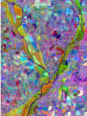
Examples/ChangeDetection/MultivariateAlterationDetector.cxx.
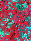
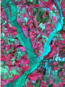
This example illustrates the class otb::MultivariateAlterationChangeDetectorImageFilter ,
which implements the Multivariate Alteration Change Detector algorithm [99]. This algorihtm allows
performing change detection from a pair multi-band images, including images with different number of
bands or modalities. Its output is a a multi-band image of change maps, each one being unccorrelated with
the remaining. The number of bands of the output image is the minimum number of bands between the two
input images.
The algorithm works as follows. It tries to find two linear combinations of bands (one for each input
images) which maximize correlation, and subtract these two linear combinitation, leading to the first change
map. Then, it looks for a second set of linear combinations which are orthogonal to the first ones, a which
maximize correlation, and use it as the second change map. This process is iterated until no more
orthogonal linear combinations can be found.
This algorithms has numerous advantages, such as radiometry scaling and shifting invariance and absence
of parameters, but it can not be used on a pair of single band images (in this case the output is simply the
difference between the two images).
We start by including the corresponding header file.
#include "otbMultivariateAlterationDetectorImageFilter.h"
We then define the types for the input images and for the change image.
typedef unsigned short InputPixelType;
typedef float OutputPixelType;
typedef otb::VectorImage<InputPixelType, Dimension> InputImageType;
typedef otb::VectorImage<OutputPixelType, Dimension> OutputImageType;
We can now declare the types for the reader. Since the images can be vey large, we will force the pipeline to
use streaming. For this purpose, the file writer will be streamed. This is achieved by using the
otb::ImageFileWriter class.
typedef otb::ImageFileReader<InputImageType> ReaderType;
typedef otb::ImageFileWriter<OutputImageType> WriterType;
typedef otb::MultivariateAlterationDetectorImageFilter<
InputImageType,OutputImageType> MADFilterType;
The different elements of the pipeline can now be instantiated.
ReaderType::Pointer reader1 = ReaderType::New(); ReaderType::Pointer reader2 = ReaderType::New();
WriterType::Pointer writer = WriterType::New(); MADFilterType::Pointer madFilter = MADFilterType::New();
We set the parameters of the different elements of the pipeline.
reader1->SetFileName(inputFilename1); reader2->SetFileName(inputFilename2);
writer->SetFileName(outputFilename);
We build the pipeline by plugging all the elements together.
madFilter->SetInput1(reader1->GetOutput()); madFilter->SetInput2(reader2->GetOutput());
writer->SetInput(madFilter->GetOutput());
And then we can trigger the pipeline update, as usual.
Figure 21.9 shows the results of Multivariate Alteration Detector applied to a pair of SPOT5 images
before and after a flooding event.