Chapter 11
Orthorectification and Map Projection

This chapter introduces the functionnalities available in OTB for image ortho-registration. We define ortho-registration as the procedure allowing to transform an image in sensor geometry to a geographic or cartographic projection.

Figure 11.1 shows a synoptic view of the different steps involved in a classical ortho-registration processing chain able to deal with image series. These steps are the following:

• Sensor modelling: the geometric sensor model allows to convert image coordinates (line, column) into geographic coordinates (latitude, longitude); a rigorous modelling needs a digital elevation model (DEM) in order to take into account the terrain topography.
• Bundle-block adjustment: in the case of image series, the geometric models and their parameters can be refined by using homologous points between the images. This is an optional step and not currently implemented in OTB.
• Map projection: this step allows to go from geographic coordinates to some specific cartographic projection as Lambert, Mercator or UTM.

11.1 Sensor Models

A sensor model is a set of equations giving the relationship between image pixel (l,c) coordinates and ground (X,Y ) coordinates for every pixel in the image. Typically, the ground coordinates are given in a geographic projection (latitude, longitude). The sensor model can be expressed either from image to ground – forward model – or from ground to image – inverse model. This can be written as follows:

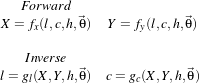
Where is the set of parameters which describe the sensor and the acquisition geometry (platform altitude, viewing angle, focal length for optical sensors, doppler centroid for SAR images, etc.).

In OTB, sensor models are implemented as itk::Transform s (see section 9.6 for details), which is the appropriate way to express coordinate changes. The base class for sensor models is otb::SensorModelBase from which the classes otb::InverseSensorModel and otb::ForwardSensorModel inherit.

As one may note from the model equations, the height of the ground, h, must be known. Usually, it means that a Digital Elevation Model, DEM, will be used.

11.1.1 Types of Sensor Models

There exists two main types of sensor models. On one hand, we have the so-called physical models, which are rigorous, complex, eventually highly non-linear equations of the sensor geometry. As such, they are difficult to inverse (obtain the inverse model from the forward one and vice-versa). They have the significant advantage of having parameters with physical meaning (angles, distances, etc.). They are specific of each sensor, which means that a library of models is required in the software. A library which has to be updated every time a new sensor is available.

On the other hand, we have general analytical models, which approximate the physical models. These models can take the form of polynomials or ratios of polynomials, the so-called rational polynomial functions or Rational Polynomial Coefficients, RPC, also known as Rapid Positioning Capability. Since they are approximations, they are less accurate than the physical models. However, the achieved accuracy is usually high: in the case of Pléiades, RPC models have errors lower than 0.02 pixels with respect to the physical model. Since these models have a standard form they are easier to use and implement. However, they have the drawback of having parameters (coefficients, actually) without physical meaning.

OTB, through the use of the OSSIM library – http://www.ossim.org – offers models for most of current sensors either through a physical or an analytical approach. This is transparent for the user, since the geometrical model for a given image is instantiated using the information stored in its meta-data. The search for a sensor model is not straightforward. It is done in 3 steps :

1. Search in the OSSIM plugin factory for a suitable model (ossimplugins::ossimPluginProjectionFactory). For instance, this factory contains Pléiades and TerraSar sensor models.
2. If no model was found, search in the OSSIM projection factory (ossimProjectionFactoryRegistry). For instance this factory contains Spot5, Landsat and Quickbird sensor models.
3. If still no model was found, search for a valid sensor model defined in an external .geom file. If no model is found, check if there are any RPC tags embedded within the image (GDAL is used to detect those RPC tags). When the tags are present, an ossimRpcModel is created.

11.1.2 Using Sensor Models

The transformation of an image in sensor geometry to geographic geometry can be done using the following steps.

1. Read image meta-data and instantiate the model with the given parameters.
2. Define the ROI in ground coordinates (this is your output pixel array)
3. Iterate through the pixels of coordinates (X,Y ):
   1. Get h from the DEM
   2. Compute (c,l) = G(X,Y,h,)
   3. Interpolate pixel values if (c,l) are not grid coordinates.

Actually, in OTB, you don’t have to manually instantiate the sensor model which is appropriate to your image. That is, you don’t have to manually choose a SPOT5 or a Quickbird sensor model. This task is automatically performed by the otb::ImageFileReader class in a similar way as the image format recognition is done. The appropriate sensor model will then be included in the image meta-data, so you can access it when needed.

The source code for this example can be found in the file
Examples/Projections/SensorModelExample.cxx.

This example illustrates how to use the sensor model read from image meta-data in order to perform ortho-rectification. This is a very basic, step-by-step example, so you understand the different components involved in the process. When performing real ortho-rectifications, you can use the example presented in section 11.3.

We will start by including the header file for the inverse sensor model.

As explained before, the first thing to do is to create the sensor model in order to transform the ground coordinates in sensor geometry coordinates. The geoetric model will automatically be created by the image file reader. So we begin by declaring the types for the input image and the image reader.

We have just instantiated the reader and set the file name, but the image data and meta-data has not yet been accessed by it. Since we need the creation of the sensor model and all the image information (size, spacing, etc.), but we do not want to read the pixel data – it could be huge – we just ask the reader to generate the output information needed.

We can now instantiate the sensor model – an inverse one, since we want to convert ground coordinates to sensor geometry. Note that the choice of the specific model (SPOT5, Ikonos, etc.) is done by the reader and we only need to instantiate a generic model.

The model is parameterized by passing to it the keyword list containing the needed information.

Since we can not be sure that the image we read actually has sensor model information, we must check for the model validity.

The types for the input and output coordinate points can be now declared. The same is done for the index types.

We will now create the output image over which we will iterate in order to transform ground coordinates to sensor coordinates and get the corresponding pixel values.

The spacing in y direction is negative since origin is the upper left corner.

We will now instantiate an extractor filter in order to get input regions by manual tiling.

Since the transformed coordinates in sensor geometry may not be integer ones, we will need an interpolator to retrieve the pixel values (note that this assumes that the input image was correctly sampled by the acquisition system).

We proceed now to create the image writer. We will also use a writer plugged to the output of the extractor filter which will write the temporary extracted regions. This is just for monitoring the process.

Since the output pixel type and the input pixel type are different, we will need to rescale the intensity values before writing them to a file.

The tricky part starts here. Note that this example is only intended for educationnal purposes and that you do not need to proceed as this. See the example in section 11.3 in order to code ortho-rectification chains in a very simple way.

You want to go on? OK. You have been warned.

We will start by declaring an image region iterator and some convenience variables.

The loop starts here.

We create an array for storing the pixel indexes.

We create an iterator for each piece of the image, and we iterate over them.

We get the current index.

We transform the index to physical coordinates.

We use the sensor model to get the pixel coordinates in the input image and we transform this coordinates to an index. Then we store the index in the array. Note that the TransformPoint() method of the model has been overloaded so that it can be used with a 3D point when the height of the ground point is known (DEM availability).

At this point, we have stored all the indexes we need for the piece of image we are processing. We can now compute the bounds of the area in the input image we need to extract.

We can now set the parameters for the extractor using a little bit of margin in order to cope with irregular geometric distortions which could be due to topography, for instance.

We give the input image to the interpolator and we loop through the index array in order to get the corresponding pixel values. Note that for every point we check whether it is inside the extracted region.

So we are done. We can now write the output image to a file after performing the intensity rescaling.

11.1.3 Evaluating Sensor Model

If no appropriate sensor model is available in the image meta-data, OTB offers the possibility to estimate a sensor model from the image.

The source code for this example can be found in the file
Examples/Projections/EstimateRPCSensorModelExample.cxx.

The following example illustrates the application of estimation of a sensor model to an image (limited to a RPC sensor model for now).

The otb::GCPsToRPCSensorModelImageFilter estimates a RPC sensor model from a list of user defined GCPs. Internally, it uses an ossimRpcSolver, which performs the estimation using the well known least-square method.

Let’s look at the minimal code required to use this algorithm. First, the following header defining the otb::GCPsToRPCSensorModelImageFilter class must be included.

We declare the image type based on a particular pixel type and dimension. In this case the float type is used for the pixels.

The otb::GCPsToRPCSensorModelImageFilter is instantiated.

We retrieve the command line parameters and put them in the correct variables. Firstly, We determine the number of GCPs set from the command line parameters and they are stored in:

• otb::Point3DType : Store the sensor point (3D ground point)
• otb::Point2DType : Pixel associated in the image (2D physical coordinates)

  Here we do not use DEM or MeanElevation. It is also possible to give a 2D ground point and use the DEM or MeanElevation to get the corresponding elevation.

Note that the otb::GCPsToRPCSensorModelImageFilter needs at least 20 GCPs to estimate a proper RPC sensor model, although no warning will be reported to the user if the number of GCPs is lower than 20. Actual estimation of the sensor model takes place in the GenerateOutputInformation() method.

The result of the RPC model estimation and the residual ground error is then save in a txt file. Note that This filter does not modify the image buffer, but only the metadata.

The output image can be now given to the otb::orthorectificationFilter . Note that this filter allows also to import GCPs from the image metadata, if any.

11.1.4 Limits of the Approach

As you may understand by now, accurate geo-referencing needs accurate DEM and also accurate sensor models and parameters. In the case where we have several images acquired over the same area by different sensors or different geometric configurations, geo-referencing (geographical coordinates) or ortho-rectification (cartographic coordinates) is not usually enough. Indeed, when working with image series we usually want to compare them (fusion, change detection, etc.) at the pixel level.

Since common DEM and sensor parameters do not allow for such an accuracy, we have to use clever strategies to improve the co-registration of the images. The classical one consists in refining the sensor parameters by taking homologous points between the images to co-register. This is called bundle block adjustment and will be implemented in coming versions of OTB.

Even if the model parameters are refined, errors due to DEM accuracy can not be eliminated. In this case, image to image registration can be applied. These approaches are presented in chapters 9 and 10.

11.2 Map Projections

Map projections describe the link between geographic coordinates and cartographic ones. So map projections allow to represent a 2-dimensional manifold of a 3-dimensional space (the Earth surface) in a 2-dimensional space (a map which used to be a sheet of paper!). This geometrical transformation doesn’t have a unique solution, so over the cartography history, every country or region in the world has been able to express the belief of being the center of the universe. In other words, every cartographic projection tries to minimize the distortions of the 3D to 2D transformation for a given point of the Earth surface¹ .

In OTB the otb::MapProjection class is derived from the itk::Transform class, so the coordinate transformation points are overloaded with map projection equations. The otb::MapProjection class is templated over the type of cartographic projection, which is provided by the OSSIM library. In order to hide the complexity of the approach, some type definitions for the more common projections are given in the file otbMapProjections.h file.

Sometimes, you don’t know at compile time what map projection you will need in your application. In this case, the otb::GenericMapProjection allow you to set the map projection at run-time by passing the WKT identification for the projection.

The source code for this example can be found in the file
Examples/Projections/MapProjectionExample.cxx.

Map projection is an important issue when working with satellite images. In the orthorectification process, converting between geographic and cartographic coordinates is a key step. In this process, everything is integrated and you don’t need to know the details.

However, sometimes, you need to go hands-on and find out the nitty-gritty details. This example shows you how to play with map projections in OTB and how to convert coordinates. In most cases, the underlying work is done by OSSIM.

First, we start by including the otbMapProjections header. In this file, over 30 projections are defined and ready to use. It is easy to add new one.

The otbGenericMapProjection enables you to instantiate a map projection from a WKT (Well Known Text) string, which is popular with OGR for example.

We retrieve the command line parameters and put them in the correct variables. The transforms are going to work with an itk::Point .

The output of this program will be saved in a text file. We also want to make sure that the precision of the digits will be enough.

We can now instantiate our first map projection. Here, it is a UTM projection. We also need to provide the information about the zone and the hemisphere for the projection. These are specific to the UTM projection.

The TransformPoint() method returns the coordinates of the point in the new projection.

We follow the same path for the Lambert93 projection:

If you followed carefully the previous examples, you’ve noticed that the target projections have been directly coded, which means that they can’t be changed at run-time. What happens if you don’t know the target projection when you’re writing the program? It can depend on some input provided by the user (image, shapefile).

In this situation, you can use the otb::GenericMapProjection . It will accept a string to set the projection. This string should be in the WKT format.

For example:

This string is then passed to the projection using the SetWkt() method.

And of course, we don’t forget to close the file:

The final output of the program should be:

You will seldom use a map projection by itself, but rather in an ortho-rectification framework. An example is given in the next section.

11.3 Orthorectification with OTB

The source code for this example can be found in the file
Examples/Projections/OrthoRectificationExample.cxx.

This example demonstrates the use of the otb::OrthoRectificationFilter . This filter is intended to orthorectify images which are in a distributor format with the appropriate meta-data describing the sensor model. In this example, we will choose to use an UTM projection for the output image.

The first step toward the use of these filters is to include the proper header files: the one for the ortho-rectification filter and the one defining the different projections available in OTB.

We will start by defining the types for the images, the image file reader and the image file writer. The writer will be a otb::ImageFileWriter which will allow us to set the number of stream divisions we want to apply when writing the output image, which can be very large.

We can now proceed to declare the type for the ortho-rectification filter. The class otb::OrthoRectificationFilter is templated over the input and the output image types as well as over the cartographic projection. We define therefore the type of the projection we want, which is an UTM projection for this case.

Now we need to instantiate the map projection, set the zone and hemisphere parameters and pass this projection to the orthorectification filter.

We then wire the input image to the orthorectification filter.

Using the user-provided information, we define the output region for the image generated by the orthorectification filter. We also define the spacing of the deformation grid where actual deformation values are estimated. Choosing a bigger deformation field spacing will speed up computation.

We can now set plug the ortho-rectification filter to the writer and set the number of tiles we want to split the output image in for the writing step.

Finally, we trigger the pipeline execution by calling the Update() method on the writer. Please note that the ortho-rectification filter is derived from the otb::StreamingResampleImageFilter in order to be able to compute the input image regions which are needed to build the output image. Since the resampler applies a geometric transformation (scale, rotation, etc.), this region computation is not trivial.

11.4 Vector data projection manipulation

The source code for this example can be found in the file
Examples/Projections/VectorDataProjectionExample.cxx.

Let’s assume that you have a KML file (hence in geographical coordinates) that you would like to superpose to some image with a specific map projection. Of course, you could use the handy ogr2ogr tool to do that, but it won’t integrate so seamlessly into your OTB application.

You can also suppose that the image on which you want to superpose the data is not in a specific map projection but a raw image from a particular sensor. Thanks to OTB, the same code below will be able to do the appropriate conversion.

This example demonstrates the use of the otb::VectorDataProjectionFilter .

Declare the vector data type that you would like to use in your application.

Declare and instantiate the vector data reader: otb::VectorDataFileReader . The call to the UpdateOutputInformation() method fill up the header information.

We need the image only to retrieve its projection information, i.e. map projection or sensor model parameters. Hence, the image pixels won’t be read, only the header information using the UpdateOutputInformation() method.

The otb::VectorDataProjectionFilter will do the work of converting the vector data coordinates. It is usually a good idea to use it when you design applications reading or saving vector data.

Information concerning the original projection of the vector data will be automatically retrieved from the metadata. Nothing else is needed from you:

Information about the target projection is retrieved directly from the image:

Finally, the result is saved into a new vector file.

It is worth noting that none of this code is specific to the vector data format. Whether you pass a shapefile, or a KML file, the correct driver will be automatically instantiated.

11.5 Geometries projection manipulation

The source code for this example can be found in the file
Examples/Projections/GeometriesProjectionExample.cxx.

Instead of using otb::VectorData to apply projections as explained in 11.4, we can also directly work on OGR data types thanks to otb::GeometriesProjectionFilter .

This example demonstrates how to proceed with this alternative set of vector data types.

Declare the geometries type that you would like to use in your application. Unlike otb::VectorData , otb::GeometriesSet is a single type for any kind of geometries set (OGR data source, or OGR layer).

First, declare and instantiate the data source otb::ogr::DataSource . Then, encapsulate this data source into a otb::GeometriesSet .

We need the image only to retrieve its projection information, i.e. map projection or sensor model parameters. Hence, the image pixels won’t be read, only the header information using the UpdateOutputInformation() method.

The otb::GeometriesProjectionFilter will do the work of converting the geometries coordinates. It is usually a good idea to use it when you design applications reading or saving vector data.

Information concerning the original projection of the vector data will be automatically retrieved from the metadata. Nothing else is needed from you:

Information about the target projection is retrieved directly from the image:

Finally, the result is saved into a new vector file. Unlike other OTB filters, otb::GeometriesProjectionFilter expects to be given a valid output geometries set where to store the result of its processing – otherwise the result will be an in-memory data source, and not stored in a file nor a data base.

Then, the processing is started by calling Update(). The actual serialization of the results is guaranteed to be completed when the output geometries set object goes out of scope, or when SyncToDisk is called.

Once again, it is worth noting that none of this code is specific to the vector data format. Whether you pass a shapefile, or a KML file, the correct driver will be automatically instantiated.

11.6 Elevation management with OTB

The source code for this example can be found in the file
Examples/IO/DEMHandlerExample.cxx.

OTB relies on OSSIM for elevation handling. Since release 3.16, there is a single configuration class otb::DEMHandler to manage elevation (in image projections or localization functions for example). This configuration is managed by the a proper instantiation and parameters setting of this class. These instantiations must be done before any call to geometric filters or functionalities. Ossim internal accesses to elevation are also configured by this class and this will ensure consistency throughout the library.

This class is a singleton, the New() method is deprecated and will be removed in future release. We need to use the Instance() method instead.

It allows configuring a directory containing DEM tiles (DTED or SRTM supported) using the OpenDEMDirectory() method. The OpenGeoidFile() method allows inputting a geoid file as well. Last, a default height above ellipsoid can be set using the SetDefaultHeightAboveEllipsoid() method.

We can now retrieve height above ellipsoid or height above Mean Sea Level (MSL) using the methods GetHeightAboveEllipsoid() and GetHeightAboveMSL(). Outputs of these methods depend on the configuration of the class otb::DEMHandler and the different cases are:

For GetHeightAboveEllipsoid():

• DEM and geoid both available: dem_value+geoid_offset
• No DEM but geoid available: geoid_offset
• DEM available, but no geoid: dem_value
• No DEM and no geoid available: default height above ellipsoid

For GetHeightAboveMSL():

• DEM and geoid both available: srtm_value
• No DEM but geoid available: 0
• DEM available, but no geoid: srtm_value
• No DEM and no geoid available: 0

Note that OSSIM internal calls for sensor modelling use the height above ellipsoid, and follow the same logic as the GetHeightAboveEllipsoid() method.

11.7 Vector data area extraction

The source code for this example can be found in the file
Examples/Projections/VectorDataExtractROIExample.cxx.

There is some vector data sets widely available on the internet. These data sets can be huge, covering an entire country, with hundreds of thousands objects.

Most of the time, you won’t be interested in the whole area and would like to focuss only on the area corresponding to your satellite image.

The otb::VectorDataExtractROI is able to extract the area corresponding to your satellite image, even if the image is still in sensor geometry (provided the sensor model is supported by OTB). Let’s see how we can do that.

This example demonstrates the use of the otb::VectorDataExtractROI .

After the usual declaration (you can check the source file for the details), we can declare the otb::VectorDataExtractROI :

Then, we need to specify the region to extract. This region is a bit special as it contains also information related to its reference system (cartographic projection or sensor model projection). We retrieve all these information from the image we gave as an input.

And finally, we can plug the filter in the pipeline: