We are soon entering the final stage of the release process, and it is about time to let you know about the new features you will find in OTB 3.14. This post is about one important tool we tried to improve in the last six months: segmentation. Of course there has been a lot of work done at the library level for this purpose, with new filters, new data structures, new tests, etc. but today I would like to present the result of this work from an end-user perspective.
“One application to segment them all …”
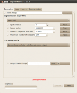
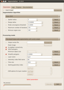
Everything that has been developed to enhance the experience of segmenting remote sensing images is packed into a single application, and I will give a tour of it in this post. For those who are not familiar with the new application framework introduced in the latest release, this is a good opportunity to catch up ! Here is what the Graphical User Interface looks like (you can launch it by typing otbgui_Segmentation on your command-line, or by clicking on the otbgui_Segmentation executable file, and even directly use the SWIG interface in python for instance). You can find detailed documentation on how to use this new application framework, as well as a complete documentation of all available applications in our CookBook.
As you can see, the application allows to apply a user-selected segmentation algorithm to the input image. The choice of segmentation algorithms includes two flavours of the MeanShift algorithm, the Watershed algorithm, as well as a simple Connected Components approach with a highly flexible connexion criterion which the user can define by entering a mathematical formula. What you can also see is that there are two different processing modes for this application. The first one, displayed in the screen capture, is to perform a standard segmentation with a raster labelled output, where each pixel is given the unique id of the segmented region it belongs to. For now, you might think that even if it is nice to have a range of segmentation algorithms in the same application, there is nothing really new there: wait for it…
Tile-based large-scale segmentation with vector output ?
The real breakthrough of this application relies in the second processing mode, called “Tile-based large-scale segmentation with vector output”. What does it mean ? In this mode, the output of the segmentation is no longer a raster, but it is a vector layer: basically any file or database table supported by OGR can be used to store the segmentation results. This vector output might be more convenient for those planning to carry on their information extraction process into a GIS software, but more importantly it removes the main blocker toward segmentation of real large remote-sensing images.
Why ? It is well known that one of the ways of getting large data processed without blowing the available memory is to process the data piece-wise (tile or strip-wise in case of images). But segmentation algorithms do not cope well with this piece-wise computation scheme, and you might also run out of available labels or end up with a raster file as large as your original input file. Moreover, the labelling of the regions depends on the layout of the tiles. If we switch from a global raster output to a global vector output, we can segment each tile one after the other, transform the labelled raster results to vector (which we do by wrapping GDAL capabilities), and dump the resulting geometries (i.e. polygons) to the output vector file or database before processing the next tile. This can hardly be done with a raster output.
So this is the major improvement in short: with the tile-based processing mode of this application, you can segment input images of arbitrary size (for instance, a Pleiades scene is 40 000 by 40 000 pixels large), it will take more time, the result will occupy more space on your hard drive, but the memory will never get saturated.
(Still) no free lunch
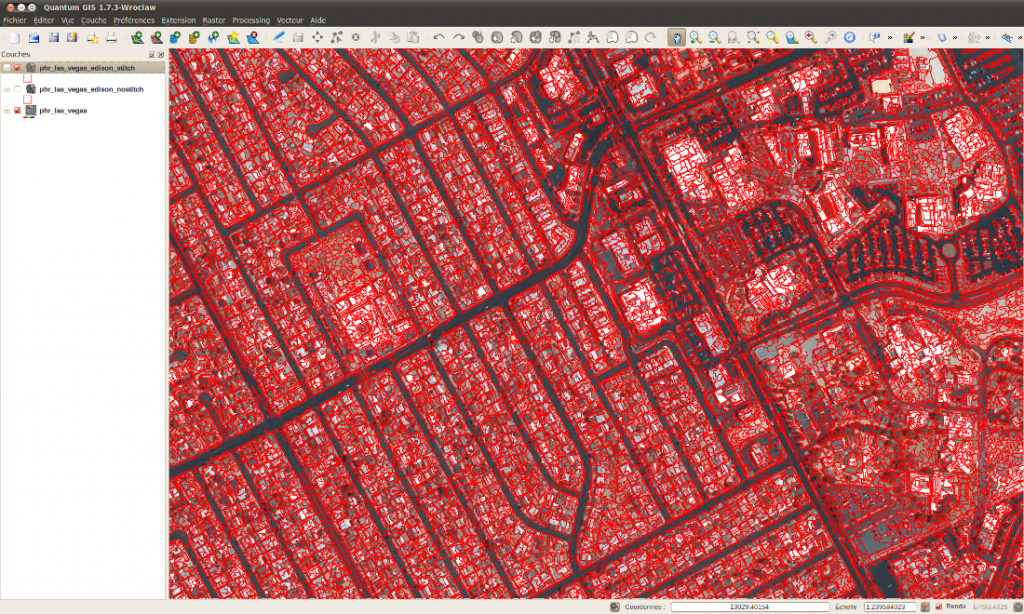
Of course, most of you will notice that if we segment on a per-tile basis, we will never get the same result as if we were segmenting the whole image at once. Objects on tile borders might get split, and regions that span over several tiles might get split into several pieces. You are right: the segmentation results obtained with this tiling scheme exhibits a lot of artefacts. To reduce this effect, we provide a simple stitching post-processing option in the application: we look for neighbouring segments on neighbouring tiles, and we merge them based on simple topological criteria. The result is of course not perfect, but it removes a lot of the tiling effect from the results.
Additional post-processing steps are available in the application: the removal of small regions (whose size is below a user-defined threshold), and the simplification of the geometries according to a given threshold. The first one is very useful to remove over-segmentation noise, while the second one is handy to reduce the output file or database size when the geometries of the segments are very complex. Finally, we offer masking capabilities to avoid segmenting areas you are not interested in.
Examples
As you may know, the application framework allows you to use the application from a graphical interface or the command-line (among others), so here is a few sample command-lines demonstrating the use of the new application. First, here is how to perform a meanshift segmentation with the classical labelled raster output:
$ otbcli_Segmentation -in input.tif -mode raster -mode.raster.out segmentation.tif uint16 -filter meanshift
To get better looking results, on can use the ColorMapping application:
$ otbcli_ColorMapping -in segmentation.tif -out segmentation_pretty.png uint8 -method optimal
An here is how to perform the same segmentation in vector mode:
$ otbcli_Segmentation -in input.tif -mode vector -mode.vector.out segmentation.shp -filter meanshift
By default, stitching of polygons is activated. To deactivate it, simply run:
$ otbcli_Segmentation -in input.tif -mode vector -mode.vector.out segmentation.shp -filter meanshift -mode.vector.stitch 0
To set the tile size to use in the tile-based segmentation, use the following option:
$ otbcli_Segmentation -in input.tif -mode vector -mode.vector.out segmentation.shp -filter meanshift -mode.vector.tilesize 1024
One can also use the application to vectorize some raster masks or raster classification results using the connected component algorithm:
$ otbcli_Segmentation -in input.tif -mode vector -mode.vector.out segmentation.shp -filter cc -filter.cc.exp "(p1b1 == 255 and p2b1 == 255)" -mode.vector.tilesize 1024
Here are some results of applying the MeanShift algorithm in vector mode on an extract of a Pleiades image displayed in QGIS, with or without stitching.
This place is bigger than our apartment!
By addressing the issue of large image segmentation, these new developments in Orfeo ToolBox set the basis for much more: large-scale object-based classification and image analysis, large scale spatial reasoning… And of course the whole framework behind can be used with any segmentation algorithm, so if you heard of some implementation of your favourite algorithm, either directly in OTB or in a licence-compatible open-source library, let us know ! We will be glad to increase the list of available algorithms. The next step we will most likely be taking in a future release will be to compute descriptors (radiometric attributes, texture information, …) from image on these segmented regions. For now, we hope you will enjoy these new features and the new applications !


