This chapter introduces the tools available in OTB for the estimation of geometric disparities between
images.
The problem we want to deal with is the one of the automatic disparity map estimation of images acquired
with different sensors. By different sensors, we mean sensors which produce images with different
radiometric properties, that is, sensors which measure different physical magnitudes: optical sensors
operating in different spectral bands, radar and optical sensors, etc.
For this kind of image pairs, the classical approach of fine correlation [82, 43], can not always be used to
provide the required accuracy, since this similarity measure (the correlation coefficient) can only measure
similarities up to an affine transformation of the radiometries.
There are two main questions which can be asked about what we want to do:
- Can we define what the similarity is between, for instance, a radar and an optical image?
- What does fine registration mean in the case where the geometric distortions are so big and
the source of information can be located in different places (for instance, the same edge can
be produced by the edge of the roof of a building in an optical image and by the wall-ground
bounce in a radar image)?
We can answer by saying that the images of the same object obtained by different sensors are two different
representations of the same reality. For the same spatial location, we have two different measures. Both
information come from the same source and thus they have a lot of common information. This
relationship may not be perfect, but it can be evaluated in a relative way: different geometrical
distortions are compared and the one leading to the strongest link between the two measures is
kept.
When working with images acquired with the same (type of) sensor one can use a very effective approach.
Since a correlation coefficient measure is robust and fast for similar images, one can afford to apply it in
every pixel of one image in order to search for the corresponding HP in the other image. One can thus build
a deformation grid (a sampling of the deformation map). If the sampling step of this grid is short enough,
the interpolation using an analytical model is not needed and high frequency deformations can be
estimated. The obtained grid can be used as a re-sampling grid and thus obtain the registered
images.
No doubt, this approach, combined with image interpolation techniques (in order to estimate sub-pixel
deformations) and multi-resolution strategies allows for obtaining the best performances in terms of
deformation estimation, and hence for the automatic image registration.
Unfortunately, in the multi-sensor case, the correlation coefficient can not be used. We will thus try to find
similarity measures which can be applied in the multi-sensor case with the same approach as the correlation
coefficient.
We start by giving several definitions which allow for the formalization of the image registration problem.
First of all, we define the master image and the slave image:
Definition 1 Master image: image to which other images will be registered; its geometry is
considered as the reference.
Definition 2 Slave image: image to be geometrically transformed in order to be registered to the
master image.
Two main concepts are the one of similarity measure and the one of geometric transformation:
Definition 3 Let I and J be two images and let c a similarity criterion, we call similarity measure any
scalar, strictly positive function
 | (10.1) |
Sc has an absolute maximum when the two images I and J are identical in the sense of the criterion
c.
Definition 4 A geometric transformation T is an operator which, applied to the coordinates (x,y)
of a point in the slave image, gives the coordinates (u,v) of its HP in the master image:
 | (10.2) |
Finally we introduce a definition for the image registration problem:
Definition 5 Registration problem:
- determine a geometric transformation T which maximizes the similarity between a master image I
and the result of the transformation T ∘J:
 | (10.3) |
- re-sampling of J by applying T .
The geometric transformation of definition 4 is used for the correction of the existing deformation between
the two images to be registered. This deformation contains information which are linked to the observed
scene and the acquisition conditions. They can be classified into 3 classes depending on their physical
source:
- deformations linked to the mean attitude of the sensor (incidence angle, presence or absence
of yaw steering, etc.);
- deformations linked to a stereo vision (mainly due to the topography);
- deformations linked to attitude evolution during the acquisition (vibrations which are mainly
present in push-broom sensors).
These deformations are characterized by their spatial frequencies and intensities which are summarized in
table 10.1.
|
|
|
| | Intensity | Spatial Frequency |
|
|
|
| Mean Attitude | Strong | Low |
|
|
|
| Stereo | Medium | High and Medium |
|
|
|
| Attitude evolution | Low | Low to Medium |
|
|
|
| |
Table 10.1: Characterization of the geometric deformation sources
Depending on the type of deformation to be corrected, its model will be different. For example, if the only
deformation to be corrected is the one introduced by the mean attitude, a physical model for the acquisition
geometry (independent of the image contents) will be enough. If the sensor is not well known,
this deformation can be approximated by a simple analytical model. When the deformations
to be modeled are high frequency, analytical (parametric) models are not suitable for a fine
registration. In this case, one has to use a fine sampling of the deformation, that means the use of
deformation grids. These grids give, for a set of pixels of the master image, their location in the slave
image.
The following points summarize the problem of the deformation modeling:
- An analytical model is just an approximation of the deformation. It is often obtained as
follows:
- Directly from a physical model without using any image content information.
- By estimation of the parameters of an a priori model (polynomial, affine, etc.). These
parameters can be estimated:
- Either by solving the equations obtained by taking HP. The HP can be manually or
automatically extracted.
- Or by maximization of a global similarity measure.
- A deformation grid is a sampling of the deformation map.
The last point implies that the sampling period of the grid must be short enough in order to
account for high frequency deformations (Shannon theorem). Of course, if the deformations
are non stationary (it is usually the case of topographic deformations), the sampling can be
irregular.
As a conclusion, we can say that definition 5 poses the registration problem as an optimization problem.
This optimization can be either global or local with a similarity measure which can also be either local or
global. All this is synthesized in table 10.2.
|
|
|
| Geometric model | Similarity measure | Optimization of the |
| | | deformation |
|
|
|
| Physical model | None | Global |
|
|
|
| Analytical model | Local | Global |
| with a priori HP | | |
|
|
|
| Analytical model | Global | Global |
| without a priori HP | | |
|
|
|
| Grid | Local | Local |
|
|
|
| |
Table 10.2: Approaches to image registration
The ideal approach would consist in a registration which is locally optimized, both in similarity and
deformation, in order to have the best registration quality. This is the case when deformation grids with
dense sampling are used. Unfortunately, this case is the most computationally heavy and one often uses
either a low sampling rate of the grid, or the evaluation of the similarity in a small set of pixels for the
estimation of an analytical model. Both of these choices lead to local registration errors which, depending
on the topography, can amount several pixels.
Even if this registration accuracy can be enough in many applications, (ortho-registration, import into a
GIS, etc.), it is not acceptable in the case of data fusion, multi-channel segmentation or change
detection [130]. This is why we will focus on the problem of deformation estimation using dense
grids.
The fine modeling of the geometric deformation we are looking for needs for the estimation of the
coordinates of nearly every pixel in the master image inside the slave image. In the classical mono-sensor
case where we use the correlation coefficient we proceed as follows.
The geometric deformation is modeled by local rigid displacements. One wants to estimate the coordinates
of each pixel of the master image inside the slave image. This can be represented by a displacement vector
associated to every pixel of the master image. Each of the two components (lines and columns) of this
vector field will be called deformation grid.
We use a small window taken in the master image and we test the similarity for every possible shift within
an exploration area inside the slave image (figure 10.1).
That means that for each position we compute the correlation coefficient. The result is a correlation surface
whose maximum gives the most likely local shift between both images:
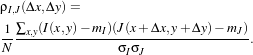 | (10.4) |
In this expression, N is the number of pixels of the analysis window, mI and mJ are the estimated mean
values inside the analysis window of respectively image I and image J and σI and σJ are their standard
deviations.
Quality criteria can be applied to the estimated maximum in order to give a confidence factor to the
estimated shift: width of the peak, maximum value, etc. Sub-pixel shifts can be measured by applying
fractional shifts to the sliding window. This can be done by image interpolation.
The interesting parameters of the procedure are:
- The size of the exploration area: it determines the computational load of the algorithm (we
want to reduce it), but it has to be large enough in order to cope with large deformations.
- The size of the sliding window: the robustness of the correlation coefficient estimation
increases with the window size, but the hypothesis of local rigid shifts may not be valid for
large windows.
The correlation coefficient cannot be used with original grey-level images in the multi-sensor case. It could
be used on extracted features (edges, etc.), but the feature extraction can introduce localization errors.
Also, when the images come from sensors using very different modalities, it can be difficult
to find similar features in both images. In this case, one can try to find the similarity at the
pixel level, but with other similarity measures and apply the same approach as we have just
described.
The concept of similarity measure has been presented in definition 3. The difficulty of the procedure
lies in finding the function f which properly represents the criterion c. We also need that f
be easily and robustly estimated with small windows. We extend here what we proposed in
[68].
We remind here the computation of the correlation coefficient between two image windows I and J. The
coordinates of the pixels inside the windows are represented by (x,y):
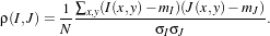 | (10.5) |
In order to qualitatively characterize the different similarity measures we propose the following
experiment. We take two images which are perfectly registered and we extract a small window of
size N ×M from each of the images (this size is set to 101×101 for this experiment). For the
master image, the window will be centered on coordinates (x0,y0) (the center of the image)
and for the slave image, it will be centered on coordinates (x0 +Δx,y0). With different values
of Δx (from -10 pixels to 10 pixels in our experiments), we obtain an estimate of ρ(I,J) as a
function of Δx, which we write as ρ(Δx) for short. The obtained curve should have a maximum
for Δx = 0, since the images are perfectly registered. We would also like to have an absolute
maximum with a high value and with a sharp peak, in order to have a good precision for the shift
estimate.
The source code for this example can be found in the file
Examples/DisparityMap/FineRegistrationImageFilterExample.cxx.
This example demonstrates the use of the otb::FineRegistrationImageFilter . This filter performs
deformation estimation using the classical extrema of image-to-image metric look-up in a search
window.
The first step toward the use of these filters is to include the proper header files.
#include "otbFineRegistrationImageFilter.h"
Several type of otb::Image are required to represent the input image, the metric field, and the
deformation field.
typedef otb::Image<PixelType, ImageDimension> InputImageType;
typedef otb::Image<PixelType, ImageDimension> MetricImageType; typedef otb::Image<DisplacementPixelType,
ImageDimension> DisplacementFieldType;
To make the metric estimation more robust, the first required step is to blur the input images. This is done
using the itk::RecursiveGaussianImageFilter :
typedef itk::RecursiveGaussianImageFilter<InputImageType, InputImageType> InputBlurType;
InputBlurType::Pointer fBlur = InputBlurType::New(); fBlur->SetInput(fReader->GetOutput());
fBlur->SetSigma(atof(argv[7])); InputBlurType::Pointer mBlur = InputBlurType::New();
mBlur->SetInput(mReader->GetOutput()); mBlur->SetSigma(atof(argv[7]));
Now, we declare and instantiate the otb::FineRegistrationImageFilter which is going to perform
the registration:
typedef otb::FineRegistrationImageFilter<InputImageType, MetricImageType, DisplacementFieldType>
RegistrationFilterType; RegistrationFilterType::Pointer registrator = RegistrationFilterType::New();
registrator->SetMovingInput(mBlur->GetOutput()); registrator->SetFixedInput(fBlur->GetOutput());
Some parameters need to be specified to the filter:
- The area where the search is performed. This area is defined by its radius:
typedef RegistrationFilterType::SizeType RadiusType; RadiusType searchRadius;
searchRadius[0] = atoi(argv[8]); searchRadius[1] = atoi(argv[8]);
registrator->SetSearchRadius(searchRadius);
- The window used to compute the local metric. This window is also defined by its radius:
RadiusType metricRadius; metricRadius[0] = atoi(argv[9]);
metricRadius[1] = atoi(argv[9]); registrator->SetRadius(metricRadius);
We need to set the sub-pixel accuracy we want to obtain:
The default matching metric used by the otb::FineRegistrationImageFilter is standard
correlation. However, we may also use any other image-to-image metric provided by ITK. For
instance, here is how we would use the itk::MutualInformationImageToImageMetric (do not
forget to include the proper header).
typedef itk::MeanReciprocalSquareDifferenceImageToImageMetric
<InputImageType, InputImageType> MRSDMetricType;
MRSDMetricType::Pointer mrsdMetric = MRSDMetricType::New(); registrator->SetMetric(mrsdMetric);
The itk::MutualInformationImageToImageMetric produces low value for poor matches,
therefore, the filter has to maximize the metric :
registrator->MinimizeOff();
The execution of the otb::FineRegistrationImageFilter will be triggered by the Update() call on
the writer at the end of the pipeline. Make sure to use a otb::ImageFileWriter if you want to benefit
from the streaming features.
Figure 10.2 shows the result of applying the otb::FineRegistrationImageFilter .
Taking figure 10.1 as a starting point, we can generalize the approach by letting the user choose:
- the similarity measure;
- the geometric transform to be estimated (see definition 4);
In order to do this, we will use the ITK registration framework locally on a set of nodes. Once the disparity
is estimated on a set of nodes, we will use it to generate a deformation field: the dense, regular vector field
which gives the translation to be applied to a pixel of the secondary image to be positioned on its
homologous point of the master image.
The source code for this example can be found in the file
Examples/DisparityMap/SimpleDisparityMapEstimationExample.cxx.
This example demonstrates the use of the otb::DisparityMapEstimationMethod , along with the
otb::NearestPointDisplacementFieldGenerator . The first filter performs deformation estimation
according to a given transform, using embedded ITK registration framework. It takes as input a
possibly non regular point set and produces a point set with associated point data representing the
deformation.
The second filter generates a deformation field by using nearest neighbor interpolation on the deformation
values from the point set. More advanced methods for deformation field interpolation are also
available.
The first step toward the use of these filters is to include the proper header files.
#include "otbDisparityMapEstimationMethod.h" #include "itkTranslationTransform.h"
#include "itkNormalizedCorrelationImageToImageMetric.h"
#include "itkWindowedSincInterpolateImageFunction.h" #include "itkGradientDescentOptimizer.h"
#include "otbBSplinesInterpolateDisplacementFieldGenerator.h" #include "itkWarpImageFilter.h"
Then we must decide what pixel type to use for the image. We choose to do all the computation
in floating point precision and rescale the results between 0 and 255 in order to export PNG
images.
typedef double PixelType; typedef unsigned char OutputPixelType;
The images are defined using the pixel type and the dimension. Please note that the
otb::NearestPointDisplacementFieldGenerator generates a otb::VectorImage to represent the
deformation field in both image directions.
typedef otb::Image<PixelType, Dimension> ImageType;
typedef otb::Image<OutputPixelType, Dimension> OutputImageType;
The next step is to define the transform we have chosen to model the deformation. In this example the
deformation is modeled as a itk::TranslationTransform .
typedef itk::TranslationTransform<double, Dimension> TransformType;
typedef TransformType::ParametersType ParametersType;
Then we define the metric we will use to evaluate the local registration between the fixed and the moving
image. In this example we chose the itk::NormalizedCorrelationImageToImageMetric
.
typedef itk::NormalizedCorrelationImageToImageMetric<ImageType, ImageType> MetricType;
Disparity map estimation implies evaluation of the moving image at non-grid position. Therefore, an
interpolator is needed. In this example we chose the itk::WindowedSincInterpolateImageFunction
.
typedef itk::Function::HammingWindowFunction<3> WindowFunctionType;
typedef itk::ZeroFluxNeumannBoundaryCondition<ImageType> ConditionType;
typedef itk::WindowedSincInterpolateImageFunction<ImageType, 3, WindowFunctionType,
ConditionType, double> InterpolatorType;
To perform local registration, an optimizer is needed. In this example we chose the
itk::GradientDescentOptimizer .
typedef itk::GradientDescentOptimizer OptimizerType;
Now we will define the point set to represent the point where to compute local disparity.
typedef itk::PointSet<ParametersType, Dimension> PointSetType;
Now we define the disparity map estimation filter.
typedef otb::DisparityMapEstimationMethod<ImageType, ImageType,
PointSetType> DMEstimationType; typedef DMEstimationType::SizeType SizeType;
The input image reader also has to be defined.
typedef otb::ImageFileReader<ImageType> ReaderType;
Two readers are instantiated : one for the fixed image, and one for the moving image.
ReaderType::Pointer fixedReader = ReaderType::New(); ReaderType::Pointer movingReader = ReaderType::New();
fixedReader->SetFileName(argv[1]); movingReader->SetFileName(argv[2]);
fixedReader->UpdateOutputInformation(); movingReader->UpdateOutputInformation();
We will the create a regular point set where to compute the local disparity.
SizeType fixedSize = fixedReader->GetOutput()->GetLargestPossibleRegion().GetSize();
unsigned int NumberOfXNodes = (fixedSize[0] - 2 ⋆ atoi(argv[7]) - 1)
/ atoi(argv[5]); unsigned int NumberOfYNodes = (fixedSize[1] - 2 ⋆ atoi(argv[7]) - 1)
/ atoi(argv[6]); ImageType::IndexType firstNodeIndex;
firstNodeIndex[0] = atoi(argv[7]); firstNodeIndex[1] = atoi(argv[7]);
PointSetType::Pointer nodes = PointSetType::New(); unsigned int nodeCounter = 0;
for (unsigned int x = 0; x < NumberOfXNodes; x++) { for (unsigned int y = 0; y < NumberOfYNodes; y++)
{ PointType p; p[0] = firstNodeIndex[0] + x⋆atoi(argv[5]);
p[1] = firstNodeIndex[1] + y⋆atoi(argv[6]); nodes->SetPoint(nodeCounter++, p); } }
We build the transform, interpolator, metric and optimizer for the disparity map estimation
filter.
TransformType::Pointer transform = TransformType::New();
OptimizerType::Pointer optimizer = OptimizerType::New(); optimizer->MinimizeOn();
optimizer->SetLearningRate(atof(argv[9])); optimizer->SetNumberOfIterations(atoi(argv[10]));
InterpolatorType::Pointer interpolator = InterpolatorType::New();
MetricType::Pointer metric = MetricType::New(); metric->SetSubtractMean(true);
We then set up the disparity map estimation filter. This filter will perform a local registration at each point
of the given point set using the ITK registration framework. It will produce a point set whose point data
reflects the disparity locally around the associated point.
Point data will contains the following data :
- The final metric value found in the registration process,
- the deformation value in the first image direction,
- the deformation value in the second image direction,
- the final parameters of the transform.
Please note that in the case of a itk::TranslationTransform , the deformation values and the transform
parameters are the same.
DMEstimationType::Pointer dmestimator = DMEstimationType::New(); dmestimator->SetTransform(transform);
dmestimator->SetOptimizer(optimizer); dmestimator->SetInterpolator(interpolator);
dmestimator->SetMetric(metric); SizeType windowSize, explorationSize;
explorationSize.Fill(atoi(argv[7])); windowSize.Fill(atoi(argv[8]));
dmestimator->SetWinSize(windowSize); dmestimator->SetExploSize(explorationSize);
The initial transform parameters can be set via the SetInitialTransformParameters() method. In our
case, we simply fill the parameter array with null values.
DMEstimationType::ParametersType initialParameters(transform->GetNumberOfParameters());
initialParameters[0] = 0.0; initialParameters[1] = 0.0;
dmestimator->SetInitialTransformParameters(initialParameters);
Now we can set the input for the deformation field estimation filter. Fixed image can be set using the
SetFixedImage() method, moving image can be set using the SetMovingImage(), and input point set can
be set using the SetPointSet() method.
dmestimator->SetFixedImage(fixedReader->GetOutput()); dmestimator->SetMovingImage(movingReader->GetOutput());
dmestimator->SetPointSet(nodes);
Once the estimation has been performed by the otb::DisparityMapEstimationMethod , one can
generate the associated deformation field (that means translation in first and second image direction). It will
be represented as a otb::VectorImage .
typedef otb::VectorImage<PixelType, Dimension> DisplacementFieldType;
For the deformation field estimation, we will use the otb::BSplinesInterpolateDisplacementFieldGenerator
. This filter will perform a nearest neighbor interpolation on the deformation values in the point set
data.
typedef otb::BSplinesInterpolateDisplacementFieldGenerator<PointSetType,
DisplacementFieldType> GeneratorType;
The disparity map estimation filter is instantiated.
GeneratorType::Pointer generator = GeneratorType::New();
We must then specify the input point set using the SetPointSet() method.
generator->SetPointSet(dmestimator->GetOutput());
One must also specify the origin, size and spacing of the output deformation field.
generator->SetOutputOrigin(fixedReader->GetOutput()->GetOrigin());
generator->SetOutputSpacing(fixedReader->GetOutput()->GetSignedSpacing());
generator->SetOutputSize(fixedReader->GetOutput() ->GetLargestPossibleRegion().GetSize());
The local registration process can lead to wrong deformation values and transform parameters. To
Select only points in point set for which the registration process was successful, one can set a
threshold on the final metric value : points for which the absolute final metric value is below
this threshold will be discarded. This threshold can be set with the SetMetricThreshold()
method.
generator->SetMetricThreshold(atof(argv[11]));
The following classes provide similar functionality:
Now we can warp our fixed image according to the estimated deformation field. This will be performed by
the itk::WarpImageFilter . First, we define this filter.
typedef itk::WarpImageFilter<ImageType, ImageType, DisplacementFieldType> ImageWarperType;
Then we instantiate it.
ImageWarperType::Pointer warper = ImageWarperType::New();
We set the input image to warp using the SetInput() method, and the deformation field using the
SetDisplacementField() method.
warper->SetInput(movingReader->GetOutput()); warper->SetDisplacementField(generator->GetOutput());
warper->SetOutputOrigin(fixedReader->GetOutput()->GetOrigin());
warper->SetOutputSpacing(fixedReader->GetOutput()->GetSignedSpacing());
In order to write the result to a PNG file, we will rescale it on a proper range.
typedef itk::RescaleIntensityImageFilter<ImageType, OutputImageType> RescalerType;
RescalerType::Pointer outputRescaler = RescalerType::New(); outputRescaler->SetInput(warper->GetOutput());
outputRescaler->SetOutputMaximum(255); outputRescaler->SetOutputMinimum(0);
We can now write the image to a file. The filters are executed by invoking the Update() method.
typedef otb::ImageFileWriter<OutputImageType> WriterType;
WriterType::Pointer outputWriter = WriterType::New(); outputWriter->SetInput(outputRescaler->GetOutput());
outputWriter->SetFileName(argv[4]); outputWriter->Update();
We also want to write the deformation field along the first direction to a file. To achieve this we will use the
otb::MultiToMonoChannelExtractROI filter.
typedef otb::MultiToMonoChannelExtractROI<PixelType, PixelType>
ChannelExtractionFilterType; ChannelExtractionFilterType::Pointer channelExtractor
= ChannelExtractionFilterType::New(); channelExtractor->SetInput(generator->GetOutput());
channelExtractor->SetChannel(1); RescalerType::Pointer fieldRescaler = RescalerType::New();
fieldRescaler->SetInput(channelExtractor->GetOutput()); fieldRescaler->SetOutputMaximum(255);
fieldRescaler->SetOutputMinimum(0); WriterType::Pointer fieldWriter = WriterType::New();
fieldWriter->SetInput(fieldRescaler->GetOutput()); fieldWriter->SetFileName(argv[3]); fieldWriter->Update();
Figure 10.3 shows the result of applying disparity map estimation on a stereo pair using a regular point set,
followed by deformation field estimation using Splines and fixed image resampling.
The source code for this example can be found in the file
Examples/DisparityMap/StereoReconstructionExample.cxx.
This example demonstrates the use of the stereo reconstruction chain from an image pair. The images are
assumed to come from the same sensor but with different positions. The approach presented here has the
following steps:
- Epipolar resampling of the image pair
- Dense disparity map estimation
- Projection of the disparities on an existing Digital Elevation Model (DEM)
It is important to note that this method requires the sensor models with a pose estimate for each
image.
#include "otbStereorectificationDisplacementFieldSource.h"
#include "otbStreamingWarpImageFilter.h" #include "otbBandMathImageFilter.h"
#include "otbSubPixelDisparityImageFilter.h" #include "otbDisparityMapMedianFilter.h"
#include "otbDisparityMapToDEMFilter.h" #include "otbImageFileReader.h"
#include "otbImageFileWriter.h" #include "otbBCOInterpolateImageFunction.h"
#include "itkUnaryFunctorImageFilter.h" #include "itkVectorCastImageFilter.h"
#include "otbImageList.h" #include "otbImageListToVectorImageFilter.h"
#include "itkRescaleIntensityImageFilter.h" #include "otbDEMHandler.h"
This example demonstrates the use of the following filters :
typedef otb::StereorectificationDisplacementFieldSource
<FloatImageType,FloatVectorImageType> DisplacementFieldSourceType;
typedef itk::Vector<double,2> DisplacementType;
typedef otb::Image<DisplacementType> DisplacementFieldType; typedef itk::VectorCastImageFilter
<FloatVectorImageType, DisplacementFieldType> DisplacementFieldCastFilterType;
typedef otb::StreamingWarpImageFilter <FloatImageType, FloatImageType,
DisplacementFieldType> WarpFilterType; typedef otb::BCOInterpolateImageFunction
<FloatImageType> BCOInterpolationType; typedef otb::Functor::NCCBlockMatching
<FloatImageType,FloatImageType> NCCBlockMatchingFunctorType;
typedef otb::PixelWiseBlockMatchingImageFilter <FloatImageType, FloatImageType, FloatImageType,
FloatImageType, NCCBlockMatchingFunctorType> NCCBlockMatchingFilterType;
typedef otb::BandMathImageFilter <FloatImageType> BandMathFilterType;
typedef otb::SubPixelDisparityImageFilter <FloatImageType, FloatImageType, FloatImageType,
FloatImageType, NCCBlockMatchingFunctorType> NCCSubPixelDisparityFilterType;
typedef otb::DisparityMapMedianFilter <FloatImageType, FloatImageType,
FloatImageType> MedianFilterType; typedef otb::DisparityMapToDEMFilter
<FloatImageType, FloatImageType, FloatImageType, FloatVectorImageType,
FloatImageType> DisparityToElevationFilterType;
The image pair is supposed to be in sensor geometry. From two images covering nearly the same area, one can
estimate a common epipolar geometry. In this geometry, an altitude variation corresponds to an horizontal
shift between the two images. The filter otb::StereorectificationDisplacementFieldSource
computes the deformation grids for each image.
These grids are sampled in epipolar geometry. They have two bands, containing the position offset (in
physical space units) between the current epipolar point and the corresponding sensor point in horizontal
and vertical direction. They can be computed at a lower resolution than sensor resolution. The application
StereoRectificationGridGenerator also provides a simple tool to generate the epipolar grids for your
image pair.
DisplacementFieldSourceType::Pointer m_DisplacementFieldSource = DisplacementFieldSourceType::New();
m_DisplacementFieldSource->SetLeftImage(leftReader->GetOutput());
m_DisplacementFieldSource->SetRightImage(rightReader->GetOutput());
m_DisplacementFieldSource->SetGridStep(4); m_DisplacementFieldSource->SetScale(1.0);
//m_DisplacementFieldSource->SetAverageElevation(avgElevation); m_DisplacementFieldSource->Update();
Then, the sensor images can be resampled in epipolar geometry, using the otb::StreamingWarpImageFilter .
The application GridBasedImageResampling also gives an easy access to this filter. The user can choose
the epipolar region to resample, as well as the resampling step and the interpolator.
Note that the epipolar image size can be retrieved from the stereo rectification grid filter.
FloatImageType::SpacingType epipolarSpacing; epipolarSpacing[0] = 1.0; epipolarSpacing[1] = 1.0;
FloatImageType::SizeType epipolarSize; epipolarSize = m_DisplacementFieldSource->GetRectifiedImageSize();
FloatImageType::PointType epipolarOrigin; epipolarOrigin[0] = 0.0;
epipolarOrigin[1] = 0.0; FloatImageType::PixelType defaultValue = 0;
The deformation grids are casted into deformation fields, then the left and right sensor images are
resampled.
DisplacementFieldCastFilterType::Pointer m_LeftDisplacementFieldCaster = DisplacementFieldCastFilterType::New();
m_LeftDisplacementFieldCaster->SetInput(m_DisplacementFieldSource->GetLeftDisplacementFieldOutput());
m_LeftDisplacementFieldCaster->GetOutput()->UpdateOutputInformation();
BCOInterpolationType::Pointer leftInterpolator = BCOInterpolationType::New();
leftInterpolator->SetRadius(2); WarpFilterType::Pointer m_LeftWarpImageFilter = WarpFilterType::New();
m_LeftWarpImageFilter->SetInput(leftReader->GetOutput());
m_LeftWarpImageFilter->SetDisplacementField(m_LeftDisplacementFieldCaster->GetOutput());
m_LeftWarpImageFilter->SetInterpolator(leftInterpolator); m_LeftWarpImageFilter->SetOutputSize(epipolarSize);
m_LeftWarpImageFilter->SetOutputSpacing(epipolarSpacing); m_LeftWarpImageFilter->SetOutputOrigin(epipolarOrigin);
m_LeftWarpImageFilter->SetEdgePaddingValue(defaultValue);
DisplacementFieldCastFilterType::Pointer m_RightDisplacementFieldCaster = DisplacementFieldCastFilterType::New();
m_RightDisplacementFieldCaster->SetInput(m_DisplacementFieldSource->GetRightDisplacementFieldOutput());
m_RightDisplacementFieldCaster->GetOutput()->UpdateOutputInformation();
BCOInterpolationType::Pointer rightInterpolator = BCOInterpolationType::New();
rightInterpolator->SetRadius(2); WarpFilterType::Pointer m_RightWarpImageFilter = WarpFilterType::New();
m_RightWarpImageFilter->SetInput(rightReader->GetOutput());
m_RightWarpImageFilter->SetDisplacementField(m_RightDisplacementFieldCaster->GetOutput());
m_RightWarpImageFilter->SetInterpolator(rightInterpolator);
m_RightWarpImageFilter->SetOutputSize(epipolarSize); m_RightWarpImageFilter->SetOutputSpacing(epipolarSpacing);
m_RightWarpImageFilter->SetOutputOrigin(epipolarOrigin); m_RightWarpImageFilter->SetEdgePaddingValue(defaultValue);
Since the resampling produces black regions around the image, it is useless to estimate disparities on these
no-data regions. We use a otb::BandMathImageFilter to produce a mask on left and right epipolar
images.
BandMathFilterType::Pointer m_LBandMathFilter = BandMathFilterType::New();
m_LBandMathFilter->SetNthInput(0,m_LeftWarpImageFilter->GetOutput(),"inleft");
#ifdef OTB_MUPARSER_HAS_CXX_LOGICAL_OPERATORS std::string leftExpr = "inleft != 0 ? 255 : 0"; #else
std::string leftExpr = "if(inleft != 0,255,0)"; #endif m_LBandMathFilter->SetExpression(leftExpr);
BandMathFilterType::Pointer m_RBandMathFilter = BandMathFilterType::New();
m_RBandMathFilter->SetNthInput(0,m_RightWarpImageFilter->GetOutput(),"inright");
#ifdef OTB_MUPARSER_HAS_CXX_LOGICAL_OPERATORS std::string rightExpr = "inright != 0 ? 255 : 0"; #else
std::string rightExpr = "if(inright != 0,255,0)"; #endif m_RBandMathFilter->SetExpression(rightExpr);
Once the two sensor images have been resampled in epipolar geometry, the disparity map can be computed.
The approach presented here is a 2D matching based on a pixel-wise metric optimization. This approach
doesn’t give the best results compared to global optimization methods, but it is suitable for streaming and
threading on large images.
The major filter used for this step is otb::PixelWiseBlockMatchingImageFilter . The metric is
computed on a window centered around the tested epipolar position. It performs a pixel-to-pixel matching
between the two epipolar images. The output disparities are given as index offset from left to right position.
The following features are available in this filter:
- Available metrics : SSD, NCC and Lp pseudo norm (computed on a square window)
- Rectangular disparity exploration area.
- Input masks for left and right images (optional).
- Output metric values (optional).
- Possibility to use input disparity estimate (as a uniform value or a full map) and an exploration
radius around these values to reduce the size of the exploration area (optional).
NCCBlockMatchingFilterType::Pointer m_NCCBlockMatcher = NCCBlockMatchingFilterType::New();
m_NCCBlockMatcher->SetLeftInput(m_LeftWarpImageFilter->GetOutput());
m_NCCBlockMatcher->SetRightInput(m_RightWarpImageFilter->GetOutput()); m_NCCBlockMatcher->SetRadius(3);
m_NCCBlockMatcher->SetMinimumHorizontalDisparity(-24); m_NCCBlockMatcher->SetMaximumHorizontalDisparity(0);
m_NCCBlockMatcher->SetMinimumVerticalDisparity(0); m_NCCBlockMatcher->SetMaximumVerticalDisparity(0);
m_NCCBlockMatcher->MinimizeOff(); m_NCCBlockMatcher->SetLeftMaskInput(m_LBandMathFilter->GetOutput());
m_NCCBlockMatcher->SetRightMaskInput(m_RBandMathFilter->GetOutput());
Some other filters have been added to enhance these pixel-to-pixel disparities. The filter
otb::SubPixelDisparityImageFilter can estimate the disparities with sub-pixel precision.
Several interpolation methods can be used : parabolic fit, triangular fit, and dichotomy search.
NCCSubPixelDisparityFilterType::Pointer m_NCCSubPixFilter = NCCSubPixelDisparityFilterType::New();
m_NCCSubPixFilter->SetInputsFromBlockMatchingFilter(m_NCCBlockMatcher);
m_NCCSubPixFilter->SetRefineMethod(NCCSubPixelDisparityFilterType::DICHOTOMY);
The filter otb::DisparityMapMedianFilter can be used to remove outliers. It has two
parameters:
- The radius of the local neighborhood to compute the median
- An incoherence threshold to reject disparities whose distance from the local median is superior
to the threshold.
MedianFilterType::Pointer m_HMedianFilter = MedianFilterType::New();
m_HMedianFilter->SetInput(m_NCCSubPixFilter->GetHorizontalDisparityOutput()); m_HMedianFilter->SetRadius(2);
m_HMedianFilter->SetIncoherenceThreshold(2.0); m_HMedianFilter->SetMaskInput(m_LBandMathFilter->GetOutput());
MedianFilterType::Pointer m_VMedianFilter = MedianFilterType::New();
m_VMedianFilter->SetInput(m_NCCSubPixFilter->GetVerticalDisparityOutput()); m_VMedianFilter->SetRadius(2);
m_VMedianFilter->SetIncoherenceThreshold(2.0); m_VMedianFilter->SetMaskInput(m_LBandMathFilter->GetOutput());
The application PixelWiseBlockMatching contains all these filters and provides a single interface to
compute your disparity maps.
The disparity map obtained with the previous step usually gives a good idea of the altitude
profile. However, it is more useful to study altitude with a DEM (Digital Elevation Model)
representation.
The filter otb::DisparityMapToDEMFilter performs this last step. The behavior of this filter is to
:
- Compute the DEM extent from the left sensor image envelope (spacing is set by the user)
- Compute the left and right rays corresponding to each valid disparity
- Compute the intersection with the mid-point method
- If the 3D point falls inside a DEM cell and has a greater elevation than the current height, the
cell height is updated
The rule of keeping the highest elevation makes sense for buildings seen from the side because the roof
edges elevation has to be kept. However this rule is not suited for noisy disparities.
The application DisparityMapToElevationMap also gives an example of use.
DisparityToElevationFilterType::Pointer m_DispToElev = DisparityToElevationFilterType::New();
m_DispToElev->SetHorizontalDisparityMapInput(m_HMedianFilter->GetOutput());
m_DispToElev->SetVerticalDisparityMapInput(m_VMedianFilter->GetOutput());
m_DispToElev->SetLeftInput(leftReader->GetOutput()); m_DispToElev->SetRightInput(rightReader->GetOutput());
m_DispToElev->SetLeftEpipolarGridInput(m_DisplacementFieldSource->GetLeftDisplacementFieldOutput());
m_DispToElev->SetRightEpipolarGridInput(m_DisplacementFieldSource->GetRightDisplacementFieldOutput());
m_DispToElev->SetElevationMin(avgElevation-10.0); m_DispToElev->SetElevationMax(avgElevation+80.0);
m_DispToElev->SetDEMGridStep(2.5); m_DispToElev->SetDisparityMaskInput(m_LBandMathFilter->GetOutput());
//m_DispToElev->SetAverageElevation(avgElevation); WriterType::Pointer m_DEMWriter = WriterType::New();
m_DEMWriter->SetInput(m_DispToElev->GetOutput()); m_DEMWriter->SetFileName(argv[3]);
m_DEMWriter->Update(); RescalerType::Pointer fieldRescaler = RescalerType::New();
fieldRescaler->SetInput(m_DispToElev->GetOutput()); fieldRescaler->SetOutputMaximum(255);
fieldRescaler->SetOutputMinimum(0); OutputWriterType::Pointer fieldWriter = OutputWriterType::New();
fieldWriter->SetInput(fieldRescaler->GetOutput()); fieldWriter->SetFileName(argv[4]); fieldWriter->Update();
Figure 10.4 shows the result of applying terrain reconstruction based using pixel-wise block matching,
sub-pixel interpolation and DEM estimation using a pair of Pleiades images over the Stadium in Toulouse,
France.