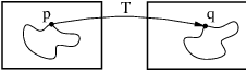
This chapter introduces OTB’s (actually mainly ITK’s) capabilities for performing image registration. Please note that the disparity map estimation approach presented in chapter 10 are very closely related to image registration. Image registration is the process of determining the spatial transform that maps points from one image to homologous points on a object in the second image. This concept is schematically represented in Figure ??. In OTB, registration is performed within a framework of pluggable components that can easily be interchanged. This flexibility means that a combinatorial variety of registration methods can be created, allowing users to pick and choose the right tools for their specific application.
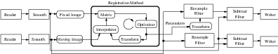
The components of the registration framework and their interconnections are shown in Figure 9.1. The basic input data to the registration process are two images: one is defined as the fixed image f(X) and the other as the moving image m(X). Where X represents a position in N-dimensional space. Registration is treated as an optimization problem with the goal of finding the spatial mapping that will bring the moving image into alignment with the fixed image.
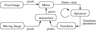
The transform component T (X) represents the spatial mapping of points from the fixed image space to points in the moving image space. The interpolator is used to evaluate moving image intensities at non-grid positions. The metric component S(f,m∘T ) provides a measure of how well the fixed image is matched by the transformed moving image. This measure forms the quantitative criterion to be optimized by the optimizer over the search space defined by the parameters of the transform.
These various OTB/ITK registration components will be described in later sections. First, we begin with some simple registration examples.
The source code for this example can be found in the file
Examples/Registration/ImageRegistration1.cxx.
This example illustrates the use of the image registration framework in ITK/OTB. It should be read as a ”Hello World” for registration. Which means that for now, you don’t ask “why?”. Instead, use the example as an introduction to the elements that are typically involved in solving an image registration problem.
A registration method requires the following set of components: two input images, a transform, a metric, an interpolator and an optimizer. Some of these components are parameterized by the image type for which the registration is intended. The following header files provide declarations of common types used for these components.
The types of each one of the components in the registration methods should be instantiated first. With that purpose, we start by selecting the image dimension and the type used for representing image pixels.
The types of the input images are instantiated by the following lines.
The transform that will map the fixed image space into the moving image space is defined below.
An optimizer is required to explore the parameter space of the transform in search of optimal values of the metric.
The metric will compare how well the two images match each other. Metric types are usually parameterized by the image types as it can be seen in the following type declaration.
Finally, the type of the interpolator is declared. The interpolator will evaluate the intensities of the moving image at non-grid positions.
The registration method type is instantiated using the types of the fixed and moving images. This class is responsible for interconnecting all the components that we have described so far.
Each one of the registration components is created using its New() method and is assigned to its respective itk::SmartPointer .
Each component is now connected to the instance of the registration method.
Since we are working with high resolution images and expected shifts are larger than the resolution, we will need to smooth the images in order to avoid the optimizer to get stucked on local minima. In order to do this, we will use a simple mean filter.
Now we can plug the output of the smoothing filters at the input of the registration method.
The registration can be restricted to consider only a particular region of the fixed image as input to the metric computation. This region is defined with the SetFixedImageRegion() method. You could use this feature to reduce the computational time of the registration or to avoid unwanted objects present in the image from affecting the registration outcome. In this example we use the full available content of the image. This region is identified by the BufferedRegion of the fixed image. Note that for this region to be valid the reader must first invoke its Update() method.
The parameters of the transform are initialized by passing them in an array. This can be used to setup an initial known correction of the misalignment. In this particular case, a translation transform is being used for the registration. The array of parameters for this transform is simply composed of the translation values along each dimension. Setting the values of the parameters to zero initializes the transform to an Identity transform. Note that the array constructor requires the number of elements to be passed as an argument.
At this point the registration method is ready for execution. The optimizer is the component that drives the execution of the registration. However, the ImageRegistrationMethod class orchestrates the ensemble to make sure that everything is in place before control is passed to the optimizer.
It is usually desirable to fine tune the parameters of the optimizer. Each optimizer has particular parameters that must be interpreted in the context of the optimization strategy it implements. The optimizer used in this example is a variant of gradient descent that attempts to prevent it from taking steps that are too large. At each iteration, this optimizer will take a step along the direction of the itk::ImageToImageMetric derivative. The initial length of the step is defined by the user. Each time the direction of the derivative abruptly changes, the optimizer assumes that a local extrema has been passed and reacts by reducing the step length by a half. After several reductions of the step length, the optimizer may be moving in a very restricted area of the transform parameter space. The user can define how small the step length should be to consider convergence to have been reached. This is equivalent to defining the precision with which the final transform should be known.
The initial step length is defined with the method SetMaximumStepLength(), while the tolerance for convergence is defined with the method SetMinimumStepLength().
In case the optimizer never succeeds reaching the desired precision tolerance, it is prudent to establish a limit on the number of iterations to be performed. This maximum number is defined with the method SetNumberOfIterations().
The registration process is triggered by an invocation to the Update() method. If something goes wrong during the initialization or execution of the registration an exception will be thrown. We should therefore place the Update() method inside a try/catch block as illustrated in the following lines.
In a real life application, you may attempt to recover from the error by taking more effective actions in the catch block. Here we are simply printing out a message and then terminating the execution of the program.
The result of the registration process is an array of parameters that defines the spatial transformation in an unique way. This final result is obtained using the GetLastTransformParameters() method.
In the case of the itk::TranslationTransform , there is a straightforward interpretation of the parameters. Each element of the array corresponds to a translation along one spatial dimension.
The optimizer can be queried for the actual number of iterations performed to reach convergence. The GetCurrentIteration() method returns this value. A large number of iterations may be an indication that the maximum step length has been set too small, which is undesirable since it results in long computational times.
The value of the image metric corresponding to the last set of parameters can be obtained with the GetValue() method of the optimizer.
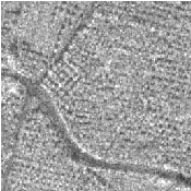
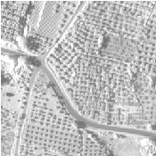
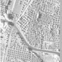
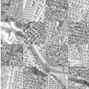
Let’s execute this example over two of the images provided in Examples/Data:
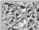
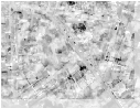
The second image is the result of intentionally translating the first image by (13,17) pixels. Both images have unit-spacing and are shown in Figure 9.2. The registration takes 18 iterations and the resulting transform parameters are:
As expected, these values match quite well the misalignment that we intentionally introduced in the moving image.
It is common, as the last step of a registration task, to use the resulting transform to map the moving image into the fixed image space. This is easily done with the itk::ResampleImageFilter . First, a ResampleImageFilter type is instantiated using the image types. It is convenient to use the fixed image type as the output type since it is likely that the transformed moving image will be compared with the fixed image.
A resampling filter is created and the moving image is connected as its input.
The Transform that is produced as output of the Registration method is also passed as input to the resampling filter. Note the use of the methods GetOutput() and Get(). This combination is needed here because the registration method acts as a filter whose output is a transform decorated in the form of a itk::DataObject . For details in this construction you may want to read the documentation of the itk::DataObjectDecorator .
The ResampleImageFilter requires additional parameters to be specified, in particular, the spacing, origin and size of the output image. The default pixel value is also set to a distinct gray level in order to highlight the regions that are mapped outside of the moving image.
The output of the filter is passed to a writer that will store the image in a file. An itk::CastImageFilter is used to convert the pixel type of the resampled image to the final type used by the writer. The cast and writer filters are instantiated below.
The filters are created by invoking their New() method.
The filters are connected together and the Update() method of the writer is invoked in order to trigger the execution of the pipeline.
The fixed image and the transformed moving image can easily be compared using the itk::SubtractImageFilter . This pixel-wise filter computes the difference between homologous pixels of its two input images.
Note that the use of subtraction as a method for comparing the images is appropriate here because we chose to represent the images using a pixel type float. A different filter would have been used if the pixel type of the images were any of the unsigned integer type.
Since the differences between the two images may correspond to very low values of intensity, we rescale those intensities with a itk::RescaleIntensityImageFilter in order to make them more visible. This rescaling will also make possible to visualize the negative values even if we save the difference image in a file format that only support unsigned pixel values1 . We also reduce the DefaultPixelValue to “1” in order to prevent that value from absorbing the dynamic range of the differences between the two images.
Its output can be passed to another writer.
For the purpose of comparison, the difference between the fixed image and the moving image before registration can also be computed by simply setting the transform to an identity transform. Note that the resampling is still necessary because the moving image does not necessarily have the same spacing, origin and number of pixels as the fixed image. Therefore a pixel-by-pixel operation cannot in general be performed. The resampling process with an identity transform will ensure that we have a representation of the moving image in the grid of the fixed image.
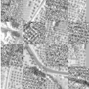
The complete pipeline structure of the current example is presented in Figure 9.4. The components of the registration method are depicted as well. Figure 9.3 (left) shows the result of resampling the moving image in order to map it onto the fixed image space. The top and right borders of the image appear in the gray level selected with the SetDefaultPixelValue() in the ResampleImageFilter. The center image shows the difference between the fixed image and the original moving image. That is, the difference before the registration is performed. The right image shows the difference between the fixed image and the transformed moving image. That is, after the registration has been performed. Both difference images have been rescaled in intensity in order to highlight those pixels where differences exist. Note that the final registration is still off by a fraction of a pixel, which results in bands around edges of anatomical structures to appear in the difference image. A perfect registration would have produced a null difference image.
This section presents a discussion on the two most common difficulties that users encounter when they start using the ITK registration framework. They are, in order of difficulty
Probably the reason why these two topics tend to create confusion is that they are implemented in different ways in other systems and therefore users tend to have different expectations regarding how things should work in OTB. The situation is further complicated by the fact that most people describe image operations as if they were manually performed in a picture in paper.
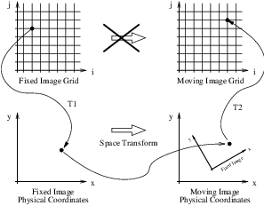
The Transform that is optimized in the ITK registration framework is the one that maps points from the physical space of the fixed image into the physical space of the moving image. This is illustrated in Figure 9.5. This implies that the Transform will accept as input points from the fixed image and it will compute the coordinates of the analogous points in the moving image. What tends to create confusion is the fact that when the Transform shifts a point on the positive X direction, the visual effect of this mapping, once the moving image is resampled, is equivalent to manually shifting the moving image along the negative X direction. In the same way, when the Transform applies a clock-wise rotation to the fixed image points, the visual effect of this mapping once the moving image has been resampled is equivalent to manually rotating the moving image counter-clock-wise.
The reason why this direction of mapping has been chosen for the ITK implementation of the registration framework is that this is the direction that better fits the fact that the moving image is expected to be resampled using the grid of the fixed image. The nature of the resampling process is such that an algorithm must go through every pixel of the fixed image and compute the intensity that should be assigned to this pixel from the mapping of the moving image. This computation involves taking the integral coordinates of the pixel in the image grid, usually called the “(i,j)” coordinates, mapping them into the physical space of the fixed image (transform T1 in Figure 9.5), mapping those physical coordinates into the physical space of the moving image (Transform to be optimized), then mapping the physical coordinates of the moving image in to the integral coordinates of the discrete grid of the moving image (transform T2 in the figure), where the value of the pixel intensity will be computed by interpolation.
If we have used the Transform that maps coordinates from the moving image physical space into the fixed image physical space, then the resampling process could not guarantee that every pixel in the grid of the fixed image was going to receive one and only one value. In other words, the resampling will have resulted in an image with holes and with redundant or overlapped pixel values.
As you have seen in the previous examples, and you will corroborate in the remaining examples in this chapter, the Transform computed by the registration framework is the Transform that can be used directly in the resampling filter in order to map the moving image into the discrete grid of the fixed image.
There are exceptional cases in which the transform that you want is actually the inverse transform of the one computed by the ITK registration framework. Only in those cases you may have to recur to invoking the GetInverse() method that most transforms offer. Make sure that before you consider following that dark path, you interact with the examples of resampling in order to get familiar with the correct interpretation of the transforms.
The second common difficulty that users encounter with the ITK registration framework is related to the fact that ITK performs registration in the context of physical space and not in the discrete space of the image grid. Figure 9.5 show this concept by crossing the transform that goes between the two image grids. One important consequence of this fact is that having the correct image origin and image pixel size is fundamental for the success of the registration process in ITK. Users must make sure that they provide correct values for the origin and spacing of both the fixed and moving images.
A typical case that helps to understand this issue, is to consider the registration of two images where one has a pixel size different from the other. For example, a SPOt 5 image and a QuickBird image. Typically a Quickbird image will have a pixel size in the order of 0.6 m, while a SPOT 5 image will have a pixel size of 2.5 m.
A user performing registration between a SPOT 5 image and a Quickbird image may be naively expecting that because the SPOT 5 image has less pixels, a scaling factor is required in the Transform in order to map this image into the Quickbird image. At that point, this person is attempting to interpret the registration process directly between the two image grids, or in pixel space. What ITK will do in this case is to take into account the pixel size that the user has provided and it will use that pixel size in order to compute a scaling factor for Transforms T1 and T2 in Figure 9.5. Since these two transforms take care of the required scaling factor, the spatial Transform to be computed during the registration process does not need to be concerned about such scaling. The transform that ITK is computing is the one that will physically map the landscape the moving image into the landscape of the fixed image.
In order to better understand this concepts, it is very useful to draw sketches of the fixed and moving image at scale in the same physical coordinate system. That is the geometrical configuration that the ITK registration framework uses as context. Keeping this in mind helps a lot for interpreting correctly the results of a registration process performed with ITK.
Some of the most challenging cases of image registration arise when images of different modalities are involved. In such cases, metrics based on direct comparison of gray levels are not applicable. It has been extensively shown that metrics based on the evaluation of mutual information are well suited for overcoming the difficulties of multi-modality registration.
The concept of Mutual Information is derived from Information Theory and its application to image registration has been proposed in different forms by different groups [28, 91, 134], a more detailed review can be found in [70]. The OTB, through ITK, currently provides five different implementations of Mutual Information metrics (see section 9.7 for details). The following example illustrates the practical use of some of these metrics.
The source code for this example can be found in the file
Examples/Registration/ImageRegistration2.cxx.
The following simple example illustrates how multiple imaging modalities can be registered using the ITK registration framework. The first difference between this and previous examples is the use of the itk::MutualInformationImageToImageMetric as the cost-function to be optimized. The second difference is the use of the itk::GradientDescentOptimizer . Due to the stochastic nature of the metric computation, the values are too noisy to work successfully with the itk::RegularStepGradientDescentOptimizer . Therefore, we will use the simpler GradientDescentOptimizer with a user defined learning rate. The following headers declare the basic components of this registration method.
One way to simplify the computation of the mutual information is to normalize the statistical distribution of the two input images. The itk::NormalizeImageFilter is the perfect tool for this task. It rescales the intensities of the input images in order to produce an output image with zero mean and unit variance.
Additionally, low-pass filtering of the images to be registered will also increase robustness against noise. In this example, we will use the itk::DiscreteGaussianImageFilter for that purpose. The characteristics of this filter have been discussed in Section 8.7.1.
The moving and fixed images types should be instantiated first.
It is convenient to work with an internal image type because mutual information will perform better on images with a normalized statistical distribution. The fixed and moving images will be normalized and converted to this internal type.
The rest of the image registration components are instantiated as illustrated in Section 9.2 with the use of the InternalImageType.
The mutual information metric type is instantiated using the image types.
The metric is created using the New() method and then connected to the registration object.
The metric requires a number of parameters to be selected, including the standard deviation of the Gaussian kernel for the fixed image density estimate, the standard deviation of the kernel for the moving image density and the number of samples use to compute the densities and entropy values. Details on the concepts behind the computation of the metric can be found in Section 9.7.4. Experience has shown that a kernel standard deviation of 0.4 works well for images which have been normalized to a mean of zero and unit variance. We will follow this empirical rule in this example.
The normalization filters are instantiated using the fixed and moving image types as input and the internal image type as output.
The blurring filters are declared using the internal image type as both the input and output types. In this example, we will set the variance for both blurring filters to 2.0.
The output of the readers becomes the input to the normalization filters. The output of the normalization filters is connected as input to the blurring filters. The input to the registration method is taken from the blurring filters.
We should now define the number of spatial samples to be considered in the metric computation. Note that we were forced to postpone this setting until we had done the preprocessing of the images because the number of samples is usually defined as a fraction of the total number of pixels in the fixed image.
The number of spatial samples can usually be as low as 1% of the total number of pixels in the fixed image. Increasing the number of samples improves the smoothness of the metric from one iteration to another and therefore helps when this metric is used in conjunction with optimizers that rely of the continuity of the metric values. The trade-off, of course, is that a larger number of samples result in longer computation times per every evaluation of the metric.
It has been demonstrated empirically that the number of samples is not a critical parameter for the registration process. When you start fine tuning your own registration process, you should start using high values of number of samples, for example in the range of 20% to 50% of the number of pixels in the fixed image. Once you have succeeded to register your images you can then reduce the number of samples progressively until you find a good compromise on the time it takes to compute one evaluation of the Metric. Note that it is not useful to have very fast evaluations of the Metric if the noise in their values results in more iterations being required by the optimizer to converge.
Since larger values of mutual information indicate better matches than smaller values, we need to maximize the cost function in this example. By default the GradientDescentOptimizer class is set to minimize the value of the cost-function. It is therefore necessary to modify its default behavior by invoking the MaximizeOn() method. Additionally, we need to define the optimizer’s step size using the SetLearningRate() method.
Note that large values of the learning rate will make the optimizer unstable. Small values, on the other hand, may result in the optimizer needing too many iterations in order to walk to the extrema of the cost function. The easy way of fine tuning this parameter is to start with small values, probably in the range of {5.0,10.0}. Once the other registration parameters have been tuned for producing convergence, you may want to revisit the learning rate and start increasing its value until you observe that the optimization becomes unstable. The ideal value for this parameter is the one that results in a minimum number of iterations while still keeping a stable path on the parametric space of the optimization. Keep in mind that this parameter is a multiplicative factor applied on the gradient of the Metric. Therefore, its effect on the optimizer step length is proportional to the Metric values themselves. Metrics with large values will require you to use smaller values for the learning rate in order to maintain a similar optimizer behavior.
Let’s execute this example over two of the images provided in Examples/Data:
The moving image after resampling is presented on the left side of Figure 9.7. The center and right figures present a checkerboard composite of the fixed and moving images before and after registration. Since the real deformation between the 2 images is not simply a shift, some registration errors remain, but the left part of the images is correctly registered.
The OTB/ITK image coordinate origin is typically located in one of the image corners (see section 5.1.4 for details). This results in counter-intuitive transform behavior when rotations and scaling are involved. Users tend to assume that rotations and scaling are performed around a fixed point at the center of the image. In order to compensate for this difference in natural interpretation, the concept of centered transforms have been introduced into the toolkit. The following sections describe the main characteristics of such transforms.
The source code for this example can be found in the file
Examples/Registration/ImageRegistration5.cxx.
This example illustrates the use of the itk::CenteredRigid2DTransform for performing rigid registration in 2D. The example code is for the most part identical to that presented in Section 9.2. The main difference is the use of the CenteredRigid2DTransform here instead of the itk::TranslationTransform .
In addition to the headers included in previous examples, the following header must also be included.
The transform type is instantiated using the code below. The only template parameter for this class is the representation type of the space coordinates.
The transform object is constructed below and passed to the registration method.
Since we are working with high resolution images and expected shifts are larger than the resolution, we will need to smooth the images in order to avoid the optimizer to get stucked on local minima. In order to do this, we will use a simple mean filter.
Now we can plug the output of the smoothing filters at the input of the registration method.
In this example, the input images are taken from readers. The code below updates the readers in order to ensure that the image parameters (size, origin and spacing) are valid when used to initialize the transform. We intend to use the center of the fixed image as the rotation center and then use the vector between the fixed image center and the moving image center as the initial translation to be applied after the rotation.
The center of rotation is computed using the origin, size and spacing of the fixed image.
The center of the moving image is computed in a similar way.
The most straightforward method of initializing the transform parameters is to configure the transform and then get its parameters with the method GetParameters(). Here we initialize the transform by passing the center of the fixed image as the rotation center with the SetCenter() method. Then the translation is set as the vector relating the center of the moving image to the center of the fixed image. This last vector is passed with the method SetTranslation().
Let’s finally initialize the rotation with a zero angle.
Now we pass the current transform’s parameters as the initial parameters to be used when the registration process starts.
Keeping in mind that the scale of units in rotation and translation is quite different, we take advantage of the scaling functionality provided by the optimizers. We know that the first element of the parameters array corresponds to the angle that is measured in radians, while the other parameters correspond to translations that are measured in the units of the spacin (pixels in our case). For this reason we use small factors in the scales associated with translations and the coordinates of the rotation center .
Next we set the normal parameters of the optimization method. In this case we are using an itk::RegularStepGradientDescentOptimizer . Below, we define the optimization parameters like the relaxation factor, initial step length, minimal step length and number of iterations. These last two act as stopping criteria for the optimization.
Let’s execute this example over two of the images provided in Examples/Data:
The second image is the result of intentionally rotating the first image by 10 degrees around the geometrical center of the image. Both images have unit-spacing and are shown in Figure 9.8. The registration takes 21 iterations and produces the results:
These results are interpreted as
As expected, these values match the misalignment intentionally introduced into the moving image quite well, since 10 degrees is about 0.174532 radians.

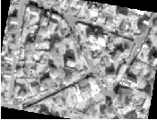
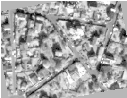
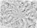
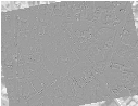
Figure 9.9 shows from left to right the resampled moving image after registration, the difference between fixed and moving images before registration, and the difference between fixed and resampled moving image after registration. It can be seen from the last difference image that the rotational component has been solved but that a small centering misalignment persists.
Let’s now consider the case in which rotations and translations are present in the initial registration, as in the following pair of images:
The second image is the result of intentionally rotating the first image by 10 degrees and then translating it 13 pixels in X and 17 pixels in Y . Both images have unit-spacing and are shown in Figure 9.10. In order to accelerate convergence it is convenient to use a larger step length as shown here.
optimizer->SetMaximumStepLength( 1.0 );
The registration now takes 34 iterations and produces the following results:
These parameters are interpreted as
These values approximately match the initial misalignment intentionally introduced into the moving image, since 10 degrees is about 0.174532 radians. The horizontal translation is well resolved while the vertical translation ends up being off by about one millimeter.
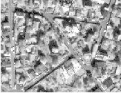
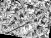
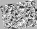

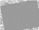
Figure 9.11 shows the output of the registration. The rightmost image of this figure shows the difference between the fixed image and the resampled moving image after registration.
The source code for this example can be found in the file
Examples/Registration/ImageRegistration9.cxx.
This example illustrates the use of the itk::AffineTransform for performing registration. The example code is, for the most part, identical to previous ones. The main difference is the use of the AffineTransform here instead of the itk::CenteredRigid2DTransform . We will focus on the most relevant changes in the current code and skip the basic elements already explained in previous examples.
Let’s start by including the header file of the AffineTransform.
We define then the types of the images to be registered.
The transform type is instantiated using the code below. The template parameters of this class are the representation type of the space coordinates and the space dimension.
The transform object is constructed below and passed to the registration method.
Since we are working with high resolution images and expected shifts are larger than the resolution, we will need to smooth the images in order to avoid the optimizer to get stucked on local minima. In order to do this, we will use a simple mean filter.
Now we can plug the output of the smoothing filters at the input of the registration method.
In this example, we use the itk::CenteredTransformInitializer helper class in order to compute a reasonable value for the initial center of rotation and the translation. The initializer is set to use the center of mass of each image as the initial correspondence correction.
Now we pass the parameters of the current transform as the initial parameters to be used when the registration process starts.
Keeping in mind that the scale of units in scaling, rotation and translation are quite different, we take advantage of the scaling functionality provided by the optimizers. We know that the first N ×N elements of the parameters array correspond to the rotation matrix factor, the next N correspond to the rotation center, and the last N are the components of the translation to be applied after multiplication with the matrix is performed.
We also set the usual parameters of the optimization method. In this case we are using an itk::RegularStepGradientDescentOptimizer . Below, we define the optimization parameters like initial step length, minimal step length and number of iterations. These last two act as stopping criteria for the optimization.
We also set the optimizer to do minimization by calling the MinimizeOn() method.
Finally we trigger the execution of the registration method by calling the Update() method. The call is placed in a try/catch block in case any exceptions are thrown.
Once the optimization converges, we recover the parameters from the registration method. This is done with the GetLastTransformParameters() method. We can also recover the final value of the metric with the GetValue() method and the final number of iterations with the GetCurrentIteration() method.
Let’s execute this example over two of the images provided in Examples/Data:
The second image is the result of intentionally rotating the first image by 10 degrees and then translating by (13,17). Both images have unit-spacing and are shown in Figure 9.12. We execute the code using the following parameters: step length=1.0, translation scale= 0.0001 and maximum number of iterations = 300. With these images and parameters the registration takes 83 iterations and produces
These results are interpreted as
The second component of the matrix values is usually associated with sinθ. We obtain the rotation through SVD of the affine matrix. The value is 10.0401 degrees, which is approximately the intentional misalignment of 10.0 degrees.


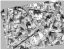
Figure 9.13 shows the output of the registration. The right most image of this figure shows the squared magnitude difference between the fixed image and the resampled moving image.
In OTB, we use the Insight Toolkit itk::Transform objects encapsulate the mapping of points and vectors from an input space to an output space. If a transform is invertible, back transform methods are also provided. Currently, ITK provides a variety of transforms from simple translation, rotation and scaling to general affine and kernel transforms. Note that, while in this section we discuss transforms in the context of registration, transforms are general and can be used for other applications. Some of the most commonly used transforms will be discussed in detail later. Let’s begin by introducing the objects used in ITK for representing basic spatial concepts.
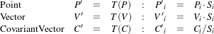
ITK implements a consistent geometric representation of the space. The characteristics of classes involved in this representation are summarized in Table 9.1. In this regard, ITK takes full advantage of the capabilities of Object Oriented programming and resists the temptation of using simple arrays of float or double in order to represent geometrical objects. The use of basic arrays would have blurred the important distinction between the different geometrical concepts and would have allowed for the innumerable conceptual and programming errors that result from using a vector where a point is needed or vice versa.
Class | Geometrical concept |
Position in space. In N-dimensional space it is represented by an array of N numbers associated with space coordinates. |
|
Relative position between two points. In N-dimensional space it is represented by an array of N numbers, each one associated with the distance along a coordinate axis. Vectors do not have a position in space. A vector is defined as the subtraction of two points. |
|
Orthogonal direction to a (N - 1)-dimensional manifold in space. For example, in 3D it corresponds to the vector orthogonal to a surface. This is the appropriate class for representing Gradients of functions. Covariant vectors do not have a position in space. Covariant vector should not be added to Points, nor to Vectors. |
|
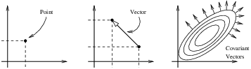
Additional uses of the itk::Point , itk::Vector and itk::CovariantVector classes have been discussed in Chapter 5. Each one of these classes behaves differently under spatial transformations. It is therefore quite important to keep their distinction clear. Figure 9.14 illustrates the differences between these concepts.
Transform classes provide different methods for mapping each one of the basic space-representation objects. Points, vectors and covariant vectors are transformed using the methods TransformPoint(), TransformVector() and TransformCovariantVector() respectively.
One of the classes that deserve further comments is the itk::Vector . This ITK class tend to be misinterpreted as a container of elements instead of a geometrical object. This is a common misconception originated by the fact that Computer Scientist and Software Engineers misuse the term “Vector”. The actual word “Vector” is relatively young. It was coined by William Hamilton in his book “Elements of Quaternions” published in 1886 (post-mortem)[55]. In the same text Hamilton coined the terms: “Scalar”, “Versor” and “Tensor”. Although the modern term of “Tensor” is used in Calculus in a different sense of what Hamilton defined in his book at the time [40].
A “Vector” is, by definition, a mathematical object that embodies the concept of “direction in space”. Strictly speaking, a Vector describes the relationship between two Points in space, and captures both their relative distance and orientation.
Computer scientists and software engineers misused the term vector in order to represent the concept of an “Indexed Set” [7]. Mechanical Engineers and Civil Engineers, who deal with the real world of physical objects will not commit this mistake and will keep the word “Vector” attached to a geometrical concept. Biologists, on the other hand, will associate “Vector” to a “vehicle” that allows them to direct something in a particular direction, for example, a virus that allows them to insert pieces of code into a DNA strand [89].
Textbooks in programming do not help to clarify those concepts and loosely use the term “Vector” for the purpose of representing an “enumerated set of common elements”. STL follows this trend and continue using the word “Vector” for what it was not supposed to be used [7, 2]. Linear algebra separates the “Vector” from its notion of geometric reality and makes it an abstract set of numbers with arithmetic operations associated.
For those of you who are looking for the “Vector” in the Software Engineering sense, please look at the itk::Array and itk::FixedArray classes that actually provide such functionalities. Additionally, the itk::VectorContainer and itk::MapContainer classes may be of interest too. These container classes are intended for algorithms that require to insert and delete elements, and that may have large numbers of elements.
The Insight Toolkit deals with real objects that inhabit the physical space. This is particularly true in the context of the image registration framework. We chose to give the appropriate name to the mathematical objects that describe geometrical relationships in N-Dimensional space. It is for this reason that we explicitly make clear the distinction between Point, Vector and CovariantVector, despite the fact that most people would be happy with a simple use of double[3] for the three concepts and then will proceed to perform all sort of conceptually flawed operations such as
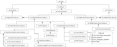
In order to enforce the correct use of the Geometrical concepts in ITK we organized these classes in a hierarchy that supports reuse of code and yet compartmentalize the behavior of the individual classes. The use of the itk::FixedArray as base class of the itk::Point , the itk::Vector and the itk::CovariantVector was a design decision based on calling things by their correct name.
An itk::FixedArray is an enumerated collection with a fixed number of elements. You can instantiate a fixed array of letters, or a fixed array of images, or a fixed array of transforms, or a fixed array of geometrical shapes. Therefore, the FixedArray only implements the functionality that is necessary to access those enumerated elements. No assumptions can be made at this point on any other operations required by the elements of the FixedArray, except the fact of having a default constructor.
The itk::Point is a type that represents the spatial coordinates of a spatial location. Based on geometrical concepts we defined the valid operations of the Point class. In particular we made sure that no operator+() was defined between Points, and that no operator⋆( scalar ) nor operator/( scalar ) were defined for Points.
In other words, you could do in ITK operations such as:
and you cannot (because you should not) do operation such as
The itk::Vector is, by Hamilton’s definition, the subtraction between two points. Therefore a Vector must satisfy the following basic operations:
An itk::Vector object is intended to be instantiated over elements that support mathematical operation such as addition, subtraction and multiplication by scalars.
Each transform class typically has several methods for setting its parameters. For example, itk::Euler2DTransform provides methods for specifying the offset, angle, and the entire rotation matrix. However, for use in the registration framework, the parameters are represented by a flat Array of doubles to facilitate communication with generic optimizers. In the case of the Euler2DTransform, the transform is also defined by three doubles: the first representing the angle, and the last two the offset. The flat array of parameters is defined using SetParameters(). A description of the parameters and their ordering is documented in the sections that follow.
In the context of registration, the transform parameters define the search space for optimizers. That is, the goal of the optimization is to find the set of parameters defining a transform that results in the best possible value of an image metric. The more parameters a transform has, the longer its computational time will be when used in a registration method since the dimension of the search space will be equal to the number of transform parameters.
Another requirement that the registration framework imposes on the transform classes is the computation of their Jacobians. In general, metrics require the knowledge of the Jacobian in order to compute Metric derivatives. The Jacobian is a matrix whose element are the partial derivatives of the output point with respect to the array of parameters that defines the transform:2
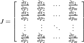 | (9.1) |
where {pi} are the transform parameters and {xi} are the coordinates of the output point. Within this framework, the Jacobian is represented by an itk::Array2D of doubles and is obtained from the transform by method GetJacobian(). The Jacobian can be interpreted as a matrix that indicates for a point in the input space how much its mapping on the output space will change as a response to a small variation in one of the transform parameters. Note that the values of the Jacobian matrix depend on the point in the input space. So actually the Jacobian can be noted as J(X), where X = {xi}. The use of transform Jacobians enables the efficient computation of metric derivatives. When Jacobians are not available, metrics derivatives have to be computed using finite difference at a price of 2M evaluations of the metric value, where M is the number of transform parameters.
The following sections describe the main characteristics of the transform classes available in ITK.
Behavior | Number of Parameters | Parameter Ordering | Restrictions |
Maps every point to itself, every vector to itself and every covariant vector to itself. | 0 | NA | Only defined when the input and output space has the same number of dimensions. |
The identity transform itk::IdentityTransform is mainly used for debugging purposes. It is provided to methods that require a transform and in cases where we want to have the certainty that the transform will have no effect whatsoever in the outcome of the process. It is just a NULL operation. The main characteristics of the identity transform are summarized in Table 9.2
Behavior | Number of Parameters | Parameter Ordering | Restrictions |
Represents a simple translation of points in the input space and has no effect on vectors or covariant vectors. | Same as the input space dimension. | The i-th parameter represents the translation in the i-th dimension. | Only defined when the input and output space has the same number of dimensions. |
The itk::TranslationTransform is probably the simplest yet one of the most useful transformations. It maps all Points by adding a Vector to them. Vector and covariant vectors remain unchanged under this transformation since they are not associated with a particular position in space. Translation is the best transform to use when starting a registration method. Before attempting to solve for rotations or scaling it is important to overlap the anatomical objects in both images as much as possible. This is done by resolving the translational misalignment between the images. Translations also have the advantage of being fast to compute and having parameters that are easy to interpret. The main characteristics of the translation transform are presented in Table 9.3.
Behavior | Number of Parameters | Parameter Ordering | Restrictions |
Points are transformed by multiplying each one of their coordinates by the corresponding scale factor for the dimension. Vectors are transformed as points. Covariant vectors are transformed by dividing their components by the scale factor in the corresponding dimension. | Same as the input space dimension. | The i-th parameter represents the scaling in the i-th dimension. | Only defined when the input and output space has the same number of dimensions. |
The itk::ScaleTransform represents a simple scaling of the vector space. Different scaling factors can be applied along each dimension. Points are transformed by multiplying each one of their coordinates by the corresponding scale factor for the dimension. Vectors are transformed in the same way as points. Covariant vectors, on the other hand, are transformed differently since anisotropic scaling does not preserve angles. Covariant vectors are transformed by dividing their components by the scale factor of the corresponding dimension. In this way, if a covariant vector was orthogonal to a vector, this orthogonality will be preserved after the transformation. The following equations summarize the effect of the transform on the basic geometric objects.
 | (9.2) |
where Pi, Vi and Ci are the point, vector and covariant vector i-th components while Si is the scaling factor along dimension i-th. The following equation illustrates the effect of the scaling transform on a 3D point.
 | (9.3) |
Scaling appears to be a simple transformation but there are actually a number of issues to keep in mind when using different scale factors along every dimension. There are subtle effects—for example, when computing image derivatives. Since derivatives are represented by covariant vectors, their values are not intuitively modified by scaling transforms.
One of the difficulties with managing scaling transforms in a registration process is that typical optimizers manage the parameter space as a vector space where addition is the basic operation. Scaling is better treated in the frame of a logarithmic space where additions result in regular multiplicative increments of the scale. Gradient descent optimizers have trouble updating step length, since the effect of an additive increment on a scale factor diminishes as the factor grows. In other words, a scale factor variation of (1.0+ϵ) is quite different from a scale variation of (5.0+ϵ).
Registrations involving scale transforms require careful monitoring of the optimizer parameters in order to keep it progressing at a stable pace. Note that some of the transforms discussed in following sections, for example, the AffineTransform, have hidden scaling parameters and are therefore subject to the same vulnerabilities of the ScaleTransform.
In cases involving misalignments with simultaneous translation, rotation and scaling components it may be desirable to solve for these components independently. The main characteristics of the scale transform are presented in Table 9.4.
Behavior | Number of Parameters | Parameter Ordering | Restrictions |
Points are transformed by multiplying each one of their coordinates by the corresponding scale factor for the dimension. Vectors are transformed as points. Covariant vectors are transformed by dividing their components by the scale factor in the corresponding dimension. | Same as the input space dimension. | The i-th parameter represents the scaling in the i-th dimension. | Only defined when the input and output space has the same number of dimensions. The difference between this transform and the ScaleTransform is that here the scaling factors are passed as logarithms, in this way their behavior is closer to the one of a Vector space. |
The itk::ScaleLogarithmicTransform is a simple variation of the itk::ScaleTransform . It is intended to improve the behavior of the scaling parameters when they are modified by optimizers. The difference between this transform and the ScaleTransform is that the parameter factors are passed here as logarithms. In this way, multiplicative variations in the scale become additive variations in the logarithm of the scaling factors.
Behavior | Number of Parameters | Parameter Ordering | Restrictions |
Represents a 2D rotation and a 2D translation. Note that the translation component has no effect on the transformation of vectors and covariant vectors. | 3 | The first parameter is the angle in radians and the last two parameters are the translation in each dimension. | Only defined for two-dimensional input and output spaces. |
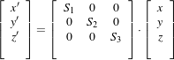
itk::Euler2DTransform implements a rigid transformation in 2D. It is composed of a plane rotation and a two-dimensional translation. The rotation is applied first, followed by the translation. The following equation illustrates the effect of this transform on a 2D point,
 | (9.4) |
where θ is the rotation angle and (T x,T y) are the components of the translation.
A challenging aspect of this transformation is the fact that translations and rotations do not form a vector space and cannot be managed as linear independent parameters. Typical optimizers make the loose assumption that parameters exist in a vector space and rely on the step length to be small enough for this assumption to hold approximately.
In addition to the non-linearity of the parameter space, the most common difficulty found when using this transform is the difference in units used for rotations and translations. Rotations are measured in radians; hence, their values are in the range [-π,π]. Translations are measured in millimeters and their actual values vary depending on the image modality being considered. In practice, translations have values on the order of 10 to 100. This scale difference between the rotation and translation parameters is undesirable for gradient descent optimizers because they deviate from the trajectories of descent and make optimization slower and more unstable. In order to compensate for these differences, ITK optimizers accept an array of scale values that are used to normalize the parameter space.
Registrations involving angles and translations should take advantage of the scale normalization functionality in order to obtain the best performance out of the optimizers. The main characteristics of the Euler2DTransform class are presented in Table 9.6.
Behavior | Number of Parameters | Parameter Ordering | Restrictions |
Represents a 2D rotation around a user-provided center followed by a 2D translation. | 5 | The first parameter is the angle in radians. Second and third are the center of rotation coordinates and the last two parameters are the translation in each dimension. | Only defined for two-dimensional input and output spaces. |
itk::CenteredRigid2DTransform implements a rigid transformation in 2D. The main difference between this transform and the itk::Euler2DTransform is that here we can specify an arbitrary center of rotation, while the Euler2DTransform always uses the origin of the coordinate system as the center of rotation. This distinction is quite important in image registration since ITK images usually have their origin in the corner of the image rather than the middle. Rotational mis-registrations usually exist, however, as rotations around the center of the image, or at least as rotations around a point in the middle of the anatomical structure captured by the image. Using gradient descent optimizers, it is almost impossible to solve non-origin rotations using a transform with origin rotations since the deep basin of the real solution is usually located across a high ridge in the topography of the cost function.
In practice, the user must supply the center of rotation in the input space, the angle of rotation and a translation to be applied after the rotation. With these parameters, the transform initializes a rotation matrix and a translation vector that together perform the equivalent of translating the center of rotation to the origin of coordinates, rotating by the specified angle, translating back to the center of rotation and finally translating by the user-specified vector.
As with the Euler2DTransform, this transform suffers from the difference in units used for rotations and translations. Rotations are measured in radians; hence, their values are in the range [-π,π]. The center of rotation and the translations are measured in millimeters, and their actual values vary depending on the image modality being considered. Registrations involving angles and translations should take advantage of the scale normalization functionality of the optimizers in order to get the best performance out of them.
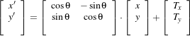
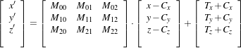
The following equation illustrates the effect of the transform on an input point (x,y) that maps to the output point (x′,y′),
 | (9.5) |
where θ is the rotation angle, (Cx,Cy) are the coordinates of the rotation center and (T x,T y) are the components of the translation. Note that the center coordinates are subtracted before the rotation and added back after the rotation. The main features of the CenteredRigid2DTransform are presented in Table 9.7.
Behavior | Number of Parameters | Parameter Ordering | Restrictions |
Represents a 2D rotation, homogeneous scaling and a 2D translation. Note that the translation component has no effect on the transformation of vectors and covariant vectors. | 4 | The first parameter is the scaling factor for all dimensions, the second is the angle in radians, and the last two parameters are the translations in (x,y) respectively. | Only defined for two-dimensional input and output spaces. |
The itk::Similarity2DTransform can be seen as a rigid transform combined with an isotropic scaling factor. This transform preserves angles between lines. In its 2D implementation, the four parameters of this transformation combine the characteristics of the itk::ScaleTransform and itk::Euler2DTransform . In particular, those relating to the non-linearity of the parameter space and the non-uniformity of the measurement units. Gradient descent optimizers should be used with caution on such parameter spaces since the notions of gradient direction and step length are ill-defined.
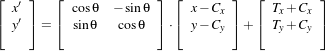
The following equation illustrates the effect of the transform on an input point (x,y) that maps to the output point (x′,y′),
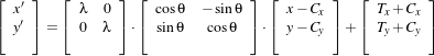 | (9.6) |
where λ is the scale factor, θ is the rotation angle, (Cx,Cy) are the coordinates of the rotation center and (T x,T y) are the components of the translation. Note that the center coordinates are subtracted before the rotation and scaling, and they are added back afterwards. The main features of the Similarity2DTransform are presented in Table 9.8.
A possible approach for controlling optimization in the parameter space of this transform is to dynamically modify the array of scales passed to the optimizer. The effect produced by the parameter scaling can be used to steer the walk in the parameter space (by giving preference to some of the parameters over others). For example, perform some iterations updating only the rotation angle, then balance the array of scale factors in the optimizer and perform another set of iterations updating only the translations.
Behavior | Number of Parameters | Parameter Ordering | Restrictions |
Represents a 3D rotation and a 3D translation. The rotation is specified as a quaternion, defined by a set of four numbers q. The relationship between quaternion and rotation about vector n by angle θ is as follows:  Note that if the quaternion is not of unit length, scaling will also result. | 7 | The first four parameters defines the quaternion and the last three parameters the translation in each dimension. | Only defined for three-dimensional input and output spaces. |
The itk::QuaternionRigidTransform class implements a rigid transformation in 3D space. The rotational part of the transform is represented using a quaternion while the translation is represented with a vector. Quaternions components do not form a vector space and hence raise the same concerns as the itk::Similarity2DTransform when used with gradient descent optimizers.
The itk::QuaternionRigidTransformGradientDescentOptimizer was introduced into the toolkit to address these concerns. This specialized optimizer implements a variation of a gradient descent algorithm adapted for a quaternion space. This class insures that after advancing in any direction on the parameter space, the resulting set of transform parameters is mapped back into the permissible set of parameters. In practice, this comes down to normalizing the newly-computed quaternion to make sure that the transformation remains rigid and no scaling is applied. The main characteristics of the QuaternionRigidTransform are presented in Table 9.9.
The Quaternion rigid transform also accepts a user-defined center of rotation. In this way, the transform can easily be used for registering images where the rotation is mostly relative to the center of the image instead one of the corners. The coordinates of this rotation center are not subject to optimization. They only participate in the computation of the mappings for Points and in the computation of the Jacobian. The transformations for Vectors and CovariantVector are not affected by the selection of the rotation center.
Behavior | Number of Parameters | Parameter Ordering | Restrictions |
Represents a 3D rotation. The rotation is specified by a versor or unit quaternion. The rotation is performed around a user-specified center of rotation. | 3 | The three parameters define the versor. | Only defined for three-dimensional input and output spaces. |
By definition, a Versor is the rotational part of a Quaternion. It can also be defined as a unit-quaternion [55, 75]. Versors only have three independent components, since they are restricted to reside in the space of unit-quaternions. The implementation of versors in the toolkit uses a set of three numbers. These three numbers correspond to the first three components of a quaternion. The fourth component of the quaternion is computed internally such that the quaternion is of unit length. The main characteristics of the itk::VersorTransform are presented in Table 9.10.
This transform exclusively represents rotations in 3D. It is intended to rapidly solve the rotational component of a more general misalignment. The efficiency of this transform comes from using a parameter space of reduced dimensionality. Versors are the best possible representation for rotations in 3D space. Sequences of versors allow the creation of smooth rotational trajectories; for this reason, they behave stably under optimization methods.
The space formed by versor parameters is not a vector space. Standard gradient descent algorithms are not appropriate for exploring this parameter space. An optimizer specialized for the versor space is available in the toolkit under the name of itk::VersorTransformOptimizer . This optimizer implements versor derivatives as originally defined by Hamilton [55].
The center of rotation can be specified by the user with the SetCenter() method. The center is not part of the parameters to be optimized, therefore it remains the same during an optimization process. Its value is used during the computations for transforming Points and when computing the Jacobian.
Behavior | Number of Parameters | Parameter Ordering | Restrictions |
Represents a 3D rotation and a 3D translation. The rotation is specified by a versor or unit quaternion, while the translation is represented by a vector. Users can specify the coordinates of the center of rotation. | 6 | The first three parameters define the versor and the last three parameters the translation in each dimension. | Only defined for three-dimensional input and output spaces. |
The itk::VersorRigid3DTransform implements a rigid transformation in 3D space. It is a variant of the itk::QuaternionRigidTransform and the itk::VersorTransform . It can be seen as a itk::VersorTransform plus a translation defined by a vector. The advantage of this class with respect to the QuaternionRigidTransform is that it exposes only six parameters, three for the versor components and three for the translational components. This reduces the search space for the optimizer to six dimensions instead of the seven dimensional used by the QuaternionRigidTransform. This transform also allows the users to set a specific center of rotation. The center coordinates are not modified during the optimization performed in a registration process. The main features of this transform are summarized in Table 9.11. This transform is probably the best option to use when dealing with rigid transformations in 3D.
Given that the space of Versors is not a Vector space, typical gradient descent optimizers are not well suited for exploring the parametric space of this transform. The itk::VersorRigid3DTransformOptimizer has been introduced in the ITK toolkit with the purpose of providing an optimizer that is aware of the Versor space properties on the rotational part of this transform, as well as the Vector space properties on the translational part of the transform.
Behavior | Number of Parameters | Parameter Ordering | Restrictions |
Represents a rigid rotation in 3D space. That is, a rotation followed by a 3D translation. The rotation is specified by three angles representing rotations to be applied around the X, Y and Z axis one after another. The translation part is represented by a Vector. Users can also specify the coordinates of the center of rotation. | 6 | The first three parameters are the rotation angles around X, Y and Z axis, and the last three parameters are the translations along each dimension. | Only defined for three-dimensional input and output spaces. |
The itk::Euler3DTransform implements a rigid transformation in 3D space. It can be seen as a rotation followed by a translation. This class exposes six parameters, three for the Euler angles that represent the rotation and three for the translational components. This transform also allows the users to set a specific center of rotation. The center coordinates are not modified during the optimization performed in a registration process. The main features of this transform are summarized in Table 9.12.
The fact that the three rotational parameters are non-linear and do not behave like Vector spaces must be taken into account when selecting an optimizer to work with this transform and when fine tuning the parameters of such optimizer. It is strongly recommended to use this transform by introducing very small variations on the rotational components. A small rotation will be in the range of 1 degree, which in radians is approximately 0.0.1745.
You should not expect this transform to be able to compensate for large rotations just by being driven with the optimizer. In practice you must provide a reasonable initialization of the transform angles and only need to correct for residual rotations in the order of 10 or 20 degrees.
Behavior | Number of Parameters | Parameter Ordering | Restrictions |
Represents a 3D rotation, a 3D translation and homogeneous scaling. The scaling factor is specified by a scalar, the rotation is specified by a versor, and the translation is represented by a vector. Users can also specify the coordinates of the center of rotation, that is the same center used for scaling. | 7 | The first parameter is the scaling factor, the next three parameters define the versor and the last three parameters the translation in each dimension. | Only defined for three-dimensional input and output spaces. |
The itk::Similarity3DTransform implements a similarity transformation in 3D space. It can be seen as an homogeneous scaling followed by a itk::VersorRigid3DTransform . This class exposes seven parameters, one for the scaling factor, three for the versor components and three for the translational components. This transform also allows the users to set a specific center of rotation. The center coordinates are not modified during the optimization performed in a registration process. Both the rotation and scaling operations are performed with respect to the center of rotation. The main features of this transform are summarized in Table 9.13.
The fact that the scaling and rotational spaces are non-linear and do not behave like Vector spaces must be taken into account when selecting an optimizer to work with this transform and when fine tuning the parameters of such optimizer.
Behavior | Number of Parameters | Parameter Ordering | Restrictions |
Represents a rigid 3D transformation followed by a perspective projection. The rotation is specified by a Versor, while the translation is represented by a Vector. Users can specify the coordinates of the center of rotation. They must specifically a focal distance to be used for the perspective projection. The rotation center and the focal distance parameters are not modified during the optimization process. | 6 | The first three parameters define the Versor and the last three parameters the Translation in each dimension. | Only defined for three-dimensional input and two-dimensional output spaces. This is one of the few transforms where the input space has a different dimension from the output space. |
The itk::Rigid3DPerspectiveTransform implements a rigid transformation in 3D space followed by a perspective projection. This transform is intended to be used in 3D∕2D registration problems where a 3D object is projected onto a 2D plane. This is the case of Fluoroscopic images used for image guided intervention, and it is also the case for classical radiography. Users must provide a value for the focal distance to be used during the computation of the perspective transform. This transform also allows users to set a specific center of rotation. The center coordinates are not modified during the optimization performed in a registration process. The main features of this transform are summarized in Table 9.14. This transform is also used when creating Digitally Reconstructed Radiographs (DRRs).
The strategies for optimizing the parameters of this transform are the same ones used for optimizing the VersorRigid3DTransform. In particular, you can use the same VersorRigid3DTranformOptimizer in order to optimize the parameters of this class.
Behavior | Number of Parameters | Parameter Ordering | Restrictions |
Represents an affine transform composed of rotation, scaling, shearing and translation. The transform is specified by a N × N matrix and a N × 1 vector where N is the space dimension. | (N +1)×N | The first N ×N parameters define the matrix in column-major order (where the column index varies the fastest). The last N parameters define the translations for each dimension. | Only defined when the input and output space have the same dimension. |
The itk::AffineTransform is one of the most popular transformations used for image registration. Its main advantage comes from the fact that it is represented as a linear transformation. The main features of this transform are presented in Table 9.15.
The set of AffineTransform coefficients can actually be represented in a vector space of dimension (N +1)×N. This makes it possible for optimizers to be used appropriately on this search space. However, the high dimensionality of the search space also implies a high computational complexity of cost-function derivatives. The best compromise in the reduction of this computational time is to use the transform’s Jacobian in combination with the image gradient for computing the cost-function derivatives.
The coefficients of the N ×N matrix can represent rotations, anisotropic scaling and shearing. These coefficients are usually of a very different dynamic range compared to the translation coefficients. Coefficients in the matrix tend to be in the range [-1 : 1], but are not restricted to this interval. Translation coefficients, on the other hand, can be on the order of 10 to 100, and are basically related to the image size and pixel spacing.
This difference in scale makes it necessary to take advantage of the functionality offered by the optimizers for rescaling the parameter space. This is particularly relevant for optimizers based on gradient descent approaches. This transform lets the user set an arbitrary center of rotation. The coordinates of the rotation center do not make part of the parameters array passed to the optimizer. Equation 9.7 illustrates the effect of applying the AffineTransform in a point in 3D space.
 | (9.7) |
A registration based on the affine transform may be more effective when applied after simpler transformations have been used to remove the major components of misalignment. Otherwise it will incur an overwhelming computational cost. For example, using an affine transform, the first set of optimization iterations would typically focus on removing large translations. This task could instead be accomplished by a translation transform in a parameter space of size N instead of the (N +1)×N associated with the affine transform.
Tracking the evolution of a registration process that uses AffineTransforms can be challenging, since it is difficult to represent the coefficients in a meaningful way. A simple printout of the transform coefficients generally does not offer a clear picture of the current behavior and trend of the optimization. A better implementation uses the affine transform to deform wire-frame cube which is shown in a 3D visualization display.
Behavior | Number of Parameters | Parameter Ordering | Restrictions |
Represents a free from deformation by providing a deformation field from the interpolation of deformations in a coarse grid. | M×N | Where M is the number of nodes in the BSpline grid and N is the dimension of the space. | Only defined when the input and output space have the same dimension. This transform has the advantage of allowing to compute deformable registration. It also has the disadvantage of having a very high dimensional parametric space, and therefore requiring long computation times. |
The itk::BSplineDeformableTransform is designed to be used for solving deformable registration problems. This transform is equivalent to generation a deformation field where a deformation vector is assigned to every point in space. The deformation vectors are computed using BSpline interpolation from the deformation values of points located in a coarse grid, that is usually referred to as the BSpline grid.
The BSplineDeformableTransform is not flexible enough for accounting for large rotations or shearing, or scaling differences. In order to compensate for this limitation, it provides the functionality of being composed with an arbitrary transform. This transform is known as the Bulk transform and it is applied to points before they are mapped with the displacement field.
This transform do not provide functionalities for mapping Vectors nor CovariantVectors, only Points can be mapped. The reason is that the variations of a vector under a deformable transform actually depend on the location of the vector in space. In other words, Vector only make sense as the relative position between two points.
The BSplineDeformableTransform has a very large number of parameters and therefore is well suited for the itk::LBFGSOptimizer and itk::LBFGSBOptimizer . The use of this transform for was proposed in the following papers [120, 93, 94].
Kernel Transforms are a set of Transforms that are also suitable for performing deformable registration. These transforms compute on the fly the displacements corresponding to a deformation field. The displacement values corresponding to every point in space are computed by interpolation from the vectors defined by a set of Source Landmarks and a set of Target Landmarks.
Several variations of these transforms are available in the toolkit. They differ on the type of interpolation kernel that is used when computing the deformation in a particular point of space. Note that these transforms are computationally expensive and that their numerical complexity is proportional to the number of landmarks and the space dimension.
The following is the list of Transforms based on the KernelTransform.
Details about the mathematical background of these transform can be found in the paper by Davis et. al [33] and the papers by Rohr et. al [117, 118].
In OTB, itk::ImageToImageMetric objects quantitatively measure how well the transformed moving image fits the fixed image by comparing the gray-scale intensity of the images. These metrics are very flexible and can work with any transform or interpolation method and do not require reduction of the gray-scale images to sparse extracted information such as edges.
The metric component is perhaps the most critical element of the registration framework. The selection of which metric to use is highly dependent on the registration problem to be solved. For example, some metrics have a large capture range while others require initialization close to the optimal position. In addition, some metrics are only suitable for comparing images obtained from the same type of sensor, while others can handle multi-sensor comparisons. Unfortunately, there are no clear-cut rules as to how to choose a metric.
The basic inputs to a metric are: the fixed and moving images, a transform and an interpolator. The method GetValue() can be used to evaluate the quantitative criterion at the transform parameters specified in the argument. Typically, the metric samples points within a defined region of the fixed image. For each point, the corresponding moving image position is computed using the transform with the specified parameters, then the interpolator is used to compute the moving image intensity at the mapped position.
The metrics also support region based evaluation. The SetFixedImageMask() and SetMovingImageMask() methods may be used to restrict evaluation of the metric within a specified region. The masks may be of any type derived from itk::SpatialObject .
Besides the measure value, gradient-based optimization schemes also require derivatives of the measure with respect to each transform parameter. The methods GetDerivatives() and GetValueAndDerivatives() can be used to obtain the gradient information.
The following is the list of metrics currently available in OTB:
In the following sections, we describe each metric type in detail. For ease of notation, we will refer to the fixed image f(X) and transformed moving image (m∘T (X)) as images A and B.
The itk::MeanSquaresImageToImageMetric computes the mean squared pixel-wise difference in intensity between image A and B over a user defined region:
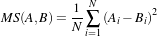 | (9.8) |
Ai is the i-th pixel of Image A
Bi is the i-th pixel of Image B
N is the number of pixels considered
The optimal value of the metric is zero. Poor matches between images A and B result in large values of the metric. This metric is simple to compute and has a relatively large capture radius.
This metric relies on the assumption that intensity representing the same homologous point must be the same in both images. Hence, its use is restricted to images of the same modality. Additionally, any linear changes in the intensity result in a poor match value.
Getting familiar with the characteristics of the Metric as a cost function is fundamental in order to find the best way of setting up an optimization process that will use this metric for solving a registration problem.
The itk::NormalizedCorrelationImageToImageMetric computes pixel-wise cross-correlation and normalizes it by the square root of the autocorrelation of the images:
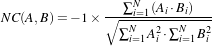 | (9.9) |
Ai is the i-th pixel of Image A
Bi is the i-th pixel of Image B
N is the number of pixels considered
Note the -1 factor in the metric computation. This factor is used to make the metric be optimal when its minimum is reached. The optimal value of the metric is then minus one. Misalignment between the images results in small measure values. The use of this metric is limited to images obtained using the same imaging modality. The metric is insensitive to multiplicative factors – illumination changes – between the two images. This metric produces a cost function with sharp peaks and well defined minima. On the other hand, it has a relatively small capture radius.
The itk::MeanReciprocalSquareDifferenceImageToImageMetric computes pixel-wise differences
and adds them after passing them through a bell-shaped function  :
:
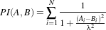 | (9.10) |
Ai is the i-th pixel of Image A
Bi is the i-th pixel of Image B
N is the number of pixels considered
λ controls the capture radius
The optimal value is N and poor matches results in small measure values. The characteristics of this metric have been studied by Penney and Holden [58][105].
This image metric has the advantage of producing poor values when few pixels are considered. This makes it consistent when its computation is subject to the size of the overlap region between the images. The capture radius of the metric can be regulated with the parameter λ. The profile of this metric is very peaky. The sharp peaks of the metric help to measure spatial misalignment with high precision. Note that the notion of capture radius is used here in terms of the intensity domain, not the spatial domain. In that regard, λ should be given in intensity units and be associated with the differences in intensity that will make drop the metric by 50%.
The metric is limited to images of the same image modality. The fact that its derivative is large at the central peak is a problem for some optimizers that rely on the derivative to decrease as the extrema are reached. This metric is also sensitive to linear changes in intensity.
The itk::MutualInformationImageToImageMetric computes the mutual information between image A and image B. Mutual information (MI) measures how much information one random variable (image intensity in one image) tells about another random variable (image intensity in the other image). The major advantage of using MI is that the actual form of the dependency does not have to be specified. Therefore, complex mapping between two images can be modeled. This flexibility makes MI well suited as a criterion of multi-modality registration [109].
Mutual information is defined in terms of entropy. Let
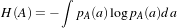 | (9.11) |
be the entropy of random variable A, H(B) the entropy of random variable B and
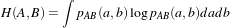 | (9.12) |
be the joint entropy of A and B. If A and B are independent, then
 | (9.13) |
and
 | (9.14) |
However, if there is any dependency, then
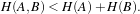 | (9.15) |
The difference is called Mutual Information : 
 | (9.16) |
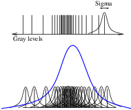
In a typical registration problem, direct access to the marginal and joint probability densities is not available and hence the densities must be estimated from the image data. Parzen windows (also known as kernel density estimators) can be used for this purpose. In this scheme, the densities are constructed by taking intensity samples S from the image and super-positioning kernel functions K(⋅) centered on the elements of S as illustrated in Figure ??:
A variety of functions can be used as the smoothing kernel with the requirement that they are smooth, symmetric, have zero mean and integrate to one. For example, boxcar, Gaussian and B-spline functions are suitable candidates. A smoothing parameter is used to scale the kernel function. The larger the smoothing parameter, the wider the kernel function used and hence the smoother the density estimate. If the parameter is too large, features such as modes in the density will get smoothed out. On the other hand, if the smoothing parameter is too small, the resulting density may be too noisy. The estimation is given by the following equation.
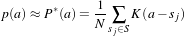 | (9.17) |
Choosing the optimal smoothing parameter is a difficult research problem and beyond the scope of this software guide. Typically, the optimal value of the smoothing parameter will depend on the data and the number of samples used.
OTB, through ITK, has multiple implementations of the mutual information metric. One of the most commonly used is itk::MutualInformationImageToImageMetric and follows the method specified by Viola and Wells in [134].
In this implementation, two separate intensity samples S and R are drawn from the image: the first to compute the density, and the second to approximate the entropy as a sample mean:
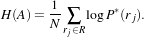 | (9.18) |
Gaussian density is used as a smoothing kernel, where the standard deviation σ acts as the smoothing parameter.
The number of spatial samples used for computation is defined using the SetNumberOfSpatialSamples() method. Typical values range from 50 to 100. Note that computation involves an N ×N loop and hence, the computation burden becomes very expensive when a large number of samples is used.
The quality of the density estimates depends on the choice of the standard deviation of the Gaussian kernel. The optimal choice will depend on the content of the images. In our experience with the toolkit, we have found that a standard deviation of 0.4 works well for images that have been normalized to have a mean of zero and standard deviation of 1.0. The standard deviation of the fixed image and moving image kernel can be set separately using methods SetFixedImageStandardDeviation() and SetMovingImageStandardDeviation().
Another form of mutual information metric available in ITK follows the method specified by Mattes et al. in [93] and is implemented by the itk::MattesMutualInformationImageToImageMetric class.
In this implementation, only one set of intensity samples is drawn from the image. Using this set, the marginal and joint probability density function (PDF) is evaluated at discrete positions or bins uniformly spread within the dynamic range of the images. Entropy values are then computed by summing over the bins.
The number of spatial samples used is set using method SetNumberOfSpatialSamples(). The number of bins used to compute the entropy values is set via SetNumberOfHistogramBins().
Since the fixed image PDF does not contribute to the metric derivatives, it does not need to be smooth. Hence, a zero order (boxcar) B-spline kernel is used for computing the PDF. On the other hand, to ensure smoothness, a third order B-spline kernel is used to compute the moving image intensity PDF. The advantage of using a B-spline kernel over a Gaussian kernel is that the B-spline kernel has a finite support region. This is computationally attractive, as each intensity sample only affects a small number of bins and hence does not require a N ×N loop to compute the metric value.
During the PDF calculations, the image intensity values are linearly scaled to have a minimum of zero and maximum of one. This rescaling means that a fixed B-spline kernel bandwidth of one can be used to handle image data with arbitrary magnitude and dynamic range.
The itk::KullbackLeiblerCompareHistogramImageToImageMetric is yet another information based metric. Kullback-Leibler distance measures the relative entropy between two discrete probability distributions. The distributions are obtained from the histograms of the two input images, A and B.
The Kullback-Liebler distance between two histograms is given by
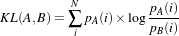 | (9.19) |
The distance is always non-negative and is zero only if the two distributions are the same. Note that the distance is not symmetric. In other words, KL(A,B)≠KL(B,A). Nevertheless, if the distributions are not too dissimilar, the difference between KL(A,B) and KL(B,A) is small.
The implementation in ITK is based on [25].
Given two images, A and B, the normalized mutual information may be computed as
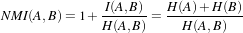 | (9.20) |
where the entropy of the images, H(A), H(B), the mutual information, I(A,B) and the joint entropy H(A,B) are computed as mentioned in 9.7.4. Details of the implementation may be found in the [54].
The itk::MeanSquaresHistogramImageToImageMetric is an alternative implementation of the Mean Squares Metric. In this implementation the joint histogram of the fixed and the mapped moving image is built first. The user selects the number of bins to use in this joint histogram. Once the joint histogram is computed, the bins are visited with an iterator. Given that each bin is associated to a pair of intensities of the form: {fixed intensity, moving intensity}, along with the number of pixels pairs in the images that fell in this bin, it is then possible to compute the sum of square distances between the intensities of both images at the quantization levels defined by the joint histogram bins.
This metric can be represented with Equation 9.21
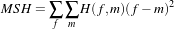 | (9.21) |
where H(f,m) is the count on the joint histogram bin identified with fixed image intensity f and moving image intensity m.
The itk::CorrelationCoefficientHistogramImageToImageMetric computes the cross correlation coefficient between the intensities in the fixed image and the intensities on the mapped moving image. This metric is intended to be used in images of the same modality where the relationship between the intensities of the fixed image and the intensities on the moving images is given by a linear equation.
The correlation coefficient is computed from the Joint histogram as
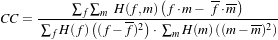 | (9.22) |
Where H(f,m) is the joint histogram count for the bin identified with the fixed image intensity f and the moving image intensity m. The values f and m are the mean values of the fixed and moving images respectively. H(f) and H(m) are the histogram counts of the fixed and moving images respectively. The optimal value of the correlation coefficient is 1, which would indicate a perfect straight line in the histogram.
The itk::MatchCardinalityImageToImageMetric computes cardinality of the set of pixels that match exactly between the moving and fixed images. In other words, it computes the number of pixel matches and mismatches between the two images. The match is designed for label maps. All pixel mismatches are considered equal whether they are between label 1 and label 2 or between label 1 and label 500. In other words, the magnitude of an individual label mismatch is not relevant, or the occurrence of a label mismatch is important.
The spatial correspondence between the fixed and moving images is established using a itk::Transform using the SetTransform() method and an interpolator using SetInterpolator(). Given that we are matching pixels with labels, it is advisable to use Nearest Neighbor interpolation.
The itk::KappaStatisticImageToImageMetric computes spatial intersection of two binary images. The metric here is designed for matching pixels in two images with the same exact value, which may be set using SetForegroundValue(). Given two images A and B, the κ coefficient is computed as
 | (9.23) |
where |A| is the number of foreground pixels in image A. This computes the fraction of area in the two images that is common to both the images. In the computation of the metric, only foreground pixels are considered.
This itk::GradientDifferenceImageToImageMetric metric evaluates the difference in the derivatives
of the moving and fixed images. The derivatives are passed through a function  and then they are added.
The purpose of this metric is to focus the registration on the edges of structures in the images. In this way
the borders exert larger influence on the result of the registration than do the inside of the homogeneous
regions on the image.
and then they are added.
The purpose of this metric is to focus the registration on the edges of structures in the images. In this way
the borders exert larger influence on the result of the registration than do the inside of the homogeneous
regions on the image.
Optimization algorithms are encapsulated as itk::Optimizer objects within OTB. Optimizers are generic and can be used for applications other than registration. Within the registration framework, subclasses of itk::SingleValuedNonLinearOptimizer are used to optimize the metric criterion with respect to the transform parameters.
The basic input to an optimizer is a cost function object. In the context of registration, itk::ImageToImageMetric classes provides this functionality. The initial parameters are set using SetInitialPosition() and the optimization algorithm is invoked by StartOptimization(). Once the optimization has finished, the final parameters can be obtained using GetCurrentPosition().
Some optimizers also allow rescaling of their individual parameters. This is convenient for normalizing parameters spaces where some parameters have different dynamic ranges. For example, the first parameter of itk::Euler2DTransform represents an angle while the last two parameters represent translations. A unit change in angle has a much greater impact on an image than a unit change in translation. This difference in scale appears as long narrow valleys in the search space making the optimization problem more difficult. Rescaling the translation parameters can help to fix this problem. Scales are represented as an itk::Array of doubles and set defined using SetScales().
There are two main types of optimizers in OTB. In the first type we find optimizers that are suitable for dealing with cost functions that return a single value. These are indeed the most common type of cost functions, and are known as Single Valued functions, therefore the corresponding optimizers are known as Single Valued optimizers. The second type of optimizers are those suitable for managing cost functions that return multiple values at each evaluation. These cost functions are common in model-fitting problems and are known as Multi Valued or Multivariate functions. The corresponding optimizers are therefore called MultipleValued optimizers in OTB.
The itk::SingleValuedNonLinearOptimizer is the base class for the first type of optimizers while the itk::MultipleValuedNonLinearOptimizer is the base class for the second type of optimizers.
The types of single valued optimizer currently available in OTB are:
A parallel hierarchy exists for optimizing multiple-valued cost functions. The base optimizer in this branch of the hierarchy is the itk::MultipleValuedNonLinearOptimizer whose only current derived class is:
Figure 9.15 illustrates the full class hierarchy of optimizers in OTB. Optimizers in the lower right corner are adaptor classes to optimizers existing in the vxl/vnl numerics toolkit. The optimizers interact with the itk::CostFunction class. In the registration framework this cost function is reimplemented in the form of ImageToImageMetric.