Segmentation of remote sensing images is a challenging task. A myriad of
different methods have been proposed and implemented in recent years. In spite of the huge effort invested
in this problem, there is no single approach that can generally solve the problem of segmentation for the
large variety of image modalities existing today.
The most effective segmentation algorithms are obtained by carefully customizing combinations of
components. The parameters of these components are tuned for the characteristics of the image modality
used as input and the features of the objects to be segmented.
The Insight Toolkit provides a basic set of algorithms that can be used to develop and customize a full
segmentation application. They are therefore available in the Orfeo Toolbox. Some of the most commonly
used segmentation components are described in the following sections.
Region growing algorithms have proven to be an effective approach for image segmentation. The basic
approach of a region growing algorithm is to start from a seed region (typically one or more pixels) that are
considered to be inside the object to be segmented. The pixels neighboring this region are evaluated to
determine if they should also be considered part of the object. If so, they are added to the region and the
process continues as long as new pixels are added to the region. Region growing algorithms vary
depending on the criteria used to decide whether a pixel should be included in the region or not,
the type connectivity used to determine neighbors, and the strategy used to visit neighboring
pixels.
Several implementations of region growing are available in ITK. This section describes some of the most
commonly used.
A simple criterion for including pixels in a growing region is to evaluate intensity value inside a specific
interval.
The source code for this example can be found in the file
Examples/Segmentation/ConnectedThresholdImageFilter.cxx.
The following example illustrates the use of the itk::ConnectedThresholdImageFilter . This filter
uses the flood fill iterator. Most of the algorithmic complexity of a region growing method comes
from visiting neighboring pixels. The flood fill iterator assumes this responsibility and greatly
simplifies the implementation of the region growing algorithm. Thus the algorithm is left to
establish a criterion to decide whether a particular pixel should be included in the current region or
not.
The criterion used by the ConnectedThresholdImageFilter is based on an interval of intensity values
provided by the user. Values of lower and upper threshold should be provided. The region growing
algorithm includes those pixels whose intensities are inside the interval.
![I(X) ∈[low er,upper]](SoftwareGuide281x.png) | (16.1) |
Let’s look at the minimal code required to use this algorithm. First, the following header defining the
ConnectedThresholdImageFilter class must be included.
#include "itkConnectedThresholdImageFilter.h"
Noise present in the image can reduce the capacity of this filter to grow large regions. When faced with
noisy images, it is usually convenient to pre-process the image by using an edge-preserving smoothing
filter. In this particular example we use the itk::CurvatureFlowImageFilter , hence we need to
include its header file.
#include "itkCurvatureFlowImageFilter.h"
We declare the image type based on a particular pixel type and dimension. In this case the float type is
used for the pixels due to the requirements of the smoothing filter.
typedef float InternalPixelType; const unsigned int Dimension = 2;
typedef otb::Image<InternalPixelType, Dimension> InternalImageType;
The smoothing filter is instantiated using the image type as a template parameter.
typedef itk::CurvatureFlowImageFilter<InternalImageType, InternalImageType> CurvatureFlowImageFilterType;
Then the filter is created by invoking the New() method and assigning the result to a itk::SmartPointer
.
CurvatureFlowImageFilterType::Pointer smoothing = CurvatureFlowImageFilterType::New();
We now declare the type of the region growing filter. In this case it is the ConnectedThresholdImageFilter.
typedef itk::ConnectedThresholdImageFilter<InternalImageType, InternalImageType> ConnectedFilterType;
Then we construct one filter of this class using the New() method.
ConnectedFilterType::Pointer connectedThreshold = ConnectedFilterType::New();
Now it is time to connect a simple, linear pipeline. A file reader is added at the beginning of the pipeline and
a cast filter and writer are added at the end. The cast filter is required to convert float pixel types to integer
types since only a few image file formats support float types.
smoothing->SetInput(reader->GetOutput()); connectedThreshold->SetInput(smoothing->GetOutput());
caster->SetInput(connectedThreshold->GetOutput()); writer->SetInput(caster->GetOutput());
The CurvatureFlowImageFilter requires a couple of parameters to be defined. The following are typical
values, however they may have to be adjusted depending on the amount of noise present in the input
image.
smoothing->SetNumberOfIterations(5); smoothing->SetTimeStep(0.125);
The ConnectedThresholdImageFilter has two main parameters to be defined. They are the lower and upper
thresholds of the interval in which intensity values should fall in order to be included in the region. Setting
these two values too close will not allow enough flexibility for the region to grow. Setting them too far apart
will result in a region that engulfs the image.
connectedThreshold->SetLower(lowerThreshold); connectedThreshold->SetUpper(upperThreshold);
The output of this filter is a binary image with zero-value pixels everywhere except on the extracted region.
The intensity value set inside the region is selected with the method SetReplaceValue()
connectedThreshold->SetReplaceValue( itk::NumericTraits<OutputPixelType>::max());
The initialization of the algorithm requires the user to provide a seed point. It is convenient to select this
point to be placed in a typical region of the structure to be segmented. The seed is passed in the form of a
itk::Index to the SetSeed() method.
connectedThreshold->SetSeed(index);
The invocation of the Update() method on the writer triggers the execution of the pipeline. It is
usually wise to put update calls in a try/catch block in case errors occur and exceptions are
thrown.
try { writer->Update(); } catch (itk::ExceptionObject& excep) {
std::cerr << "Exception caught !" << std::endl; std::cerr << excep << std::endl; }
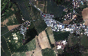
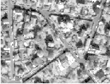
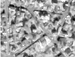
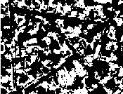
Let’s run this example using as input the image QB_Suburb.png provided in the directory Examples/Data.
We can easily segment the major structures by providing seeds in the appropriate locations and defining
values for the lower and upper thresholds. Figure 16.1 illustrates several examples of segmentation. The
parameters used are presented in Table 16.1.
|
|
|
|
|
| Structure | Seed Index | Lower | Upper | Output Image |
|
|
|
|
|
| Road | (110,38) | 50 | 100 | Second from left in Figure 16.1 |
|
|
|
|
|
| Shadow | (118,100) | 0 | 10 | Third from left in Figure 16.1 |
|
|
|
|
|
| Building | (169,146) | 220 | 255 | Fourth from left in Figure 16.1 |
|
|
|
|
|
| |
Notice that some objects are not being completely segmented. This illustrates the vulnerability of the region
growing methods when the structures to be segmented do not have a homogeneous statistical distribution
over the image space. You may want to experiment with different values of the lower and upper thresholds
to verify how the accepted region will extend.
Another option for segmenting regions is to take advantage of the functionality provided by the
ConnectedThresholdImageFilter for managing multiple seeds. The seeds can be passed one by one to the
filter using the AddSeed() method. You could imagine a user interface in which an operator clicks on
multiple points of the object to be segmented and each selected point is passed as a seed to this
filter.
Another criterion for classifying pixels is to minimize the error of misclassification. The goal is
to find a threshold that classifies the image into two clusters such that we minimize the area
under the histogram for one cluster that lies on the other cluster’s side of the threshold. This is
equivalent to minimizing the within class variance or equivalently maximizing the between class
variance.
The source code for this example can be found in the file
Examples/Segmentation/OtsuThresholdImageFilter.cxx.
This example illustrates how to use the itk::OtsuThresholdImageFilter .
#include "itkOtsuThresholdImageFilter.h"
The next step is to decide which pixel types to use for the input and output images.
typedef unsigned char InputPixelType; typedef unsigned char OutputPixelType;
The input and output image types are now defined using their respective pixel types and dimensions.
typedef otb::Image<InputPixelType, 2> InputImageType; typedef otb::Image<OutputPixelType, 2> OutputImageType;
The filter type can be instantiated using the input and output image types defined above.
typedef itk::OtsuThresholdImageFilter< InputImageType, OutputImageType> FilterType;
An otb::ImageFileReader class is also instantiated in order to read image data from a file. (See Section
6 on page 149 for more information about reading and writing data.)
typedef otb::ImageFileReader<InputImageType> ReaderType;
An otb::ImageFileWriter is instantiated in order to write the output image to a file.
typedef otb::ImageFileWriter<InputImageType> WriterType;
Both the filter and the reader are created by invoking their New() methods and assigning the result to
itk::SmartPointer s.
ReaderType::Pointer reader = ReaderType::New(); FilterType::Pointer filter = FilterType::New();
The image obtained with the reader is passed as input to the OtsuThresholdImageFilter.
filter->SetInput(reader->GetOutput());
The method SetOutsideValue() defines the intensity value to be assigned to those pixels
whose intensities are outside the range defined by the lower and upper thresholds. The method
SetInsideValue() defines the intensity value to be assigned to pixels with intensities falling inside the
threshold range.
filter->SetOutsideValue(outsideValue); filter->SetInsideValue(insideValue);
The method SetNumberOfHistogramBins() defines the number of bins to be used for computing the
histogram. This histogram will be used internally in order to compute the Otsu threshold.
filter->SetNumberOfHistogramBins(128);
The execution of the filter is triggered by invoking the Update() method. If the filter’s output has been
passed as input to subsequent filters, the Update() call on any posterior filters in the pipeline will indirectly
trigger the update of this filter.
We print out here the Threshold value that was computed internally by the filter. For this we invoke the
GetThreshold method.
int threshold = filter->GetThreshold(); std::cout << "Threshold = " << threshold << std::endl;
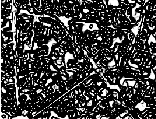
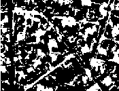
Figure 16.2 illustrates the effect of this filter. This figure shows the limitations of this filter for performing
segmentation by itself. These limitations are particularly noticeable in noisy images and in images lacking
spatial uniformity.
The following classes provide similar functionality:
The source code for this example can be found in the file
Examples/Segmentation/OtsuMultipleThresholdImageFilter.cxx.
This example illustrates how to use the itk::OtsuMultipleThresholdsCalculator .
#include "itkOtsuMultipleThresholdsCalculator.h"
OtsuMultipleThresholdsCalculator calculates thresholds for a give histogram so as to maximize the
between-class variance. We use ScalarImageToHistogramGenerator to generate histograms
typedef itk::Statistics::ScalarImageToHistogramGenerator<InputImageType>
ScalarImageToHistogramGeneratorType; typedef itk::OtsuMultipleThresholdsCalculator<
ScalarImageToHistogramGeneratorType::HistogramType> CalculatorType;
Once thresholds are computed we will use BinaryThresholdImageFilter to segment the input image into
segments.
typedef itk::BinaryThresholdImageFilter<InputImageType, OutputImageType> FilterType;
ScalarImageToHistogramGeneratorType::Pointer scalarImageToHistogramGenerator =
ScalarImageToHistogramGeneratorType::New(); CalculatorType::Pointer calculator = CalculatorType::New();
FilterType::Pointer filter = FilterType::New();
scalarImageToHistogramGenerator->SetNumberOfBins(128); int nbThresholds = argc - 2;
calculator->SetNumberOfThresholds(nbThresholds);
The pipeline will look as follows:
scalarImageToHistogramGenerator->SetInput(reader->GetOutput());
calculator->SetInputHistogram(scalarImageToHistogramGenerator->GetOutput());
filter->SetInput(reader->GetOutput()); writer->SetInput(filter->GetOutput());
Thresholds are obtained using the GetOutput method
const CalculatorType::OutputType& thresholdVector = calculator->GetOutput();
CalculatorType::OutputType::const_iterator itNum = thresholdVector.begin();
for (; itNum < thresholdVector.end(); itNum++) { std::cout << "OtsuThreshold["
<< (int) (itNum - thresholdVector.begin()) << "] = " <<
static_cast<itk::NumericTraits<CalculatorType::MeasurementType>::PrintType> (⋆itNum) << std::endl;
upperThreshold = (⋆itNum); filter->SetLowerThreshold(static_cast<OutputPixelType> (lowerThreshold));
filter->SetUpperThreshold(static_cast<OutputPixelType> (upperThreshold));
lowerThreshold = upperThreshold; writer->SetFileName(argv[2 + counter]); ++counter;
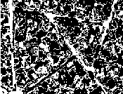
Figure 16.3 illustrates the effect of this filter.
The following classes provide similar functionality:
The source code for this example can be found in the file
Examples/Segmentation/NeighborhoodConnectedImageFilter.cxx.
The following example illustrates the use of the itk::NeighborhoodConnectedImageFilter . This
filter is a close variant of the itk::ConnectedThresholdImageFilter . On one hand, the
ConnectedThresholdImageFilter accepts a pixel in the region if its intensity is in the interval defined by two
user-provided threshold values. The NeighborhoodConnectedImageFilter, on the other hand,
will only accept a pixel if all its neighbors have intensities that fit in the interval. The size of
the neighborhood to be considered around each pixel is defined by a user-provided integer
radius.
The reason for considering the neighborhood intensities instead of only the current pixel intensity is
that small structures are less likely to be accepted in the region. The operation of this filter is
equivalent to applying the ConnectedThresholdImageFilter followed by mathematical morphology
erosion using a structuring element of the same shape as the neighborhood provided to the
NeighborhoodConnectedImageFilter.
#include "itkNeighborhoodConnectedImageFilter.h"
The itk::CurvatureFlowImageFilter is used here to smooth the image while preserving
edges.
#include "itkCurvatureFlowImageFilter.h"
We now define the image type using a particular pixel type and image dimension. In this case the float
type is used for the pixels due to the requirements of the smoothing filter.
typedef float InternalPixelType; const unsigned int Dimension = 2;
typedef otb::Image<InternalPixelType, Dimension> InternalImageType;
The smoothing filter type is instantiated using the image type as a template parameter.
typedef itk::CurvatureFlowImageFilter<InternalImageType, InternalImageType> CurvatureFlowImageFilterType;
Then, the filter is created by invoking the New() method and assigning the result to a itk::SmartPointer
.
CurvatureFlowImageFilterType::Pointer smoothing = CurvatureFlowImageFilterType::New();
We now declare the type of the region growing filter. In this case it is the NeighborhoodConnectedImageFilter.
typedef itk::NeighborhoodConnectedImageFilter<InternalImageType, InternalImageType> ConnectedFilterType;
One filter of this class is constructed using the New() method.
ConnectedFilterType::Pointer neighborhoodConnected = ConnectedFilterType::New();
Now it is time to create a simple, linear data processing pipeline. A file reader is added at the beginning
of the pipeline and a cast filter and writer are added at the end. The cast filter is required to
convert float pixel types to integer types since only a few image file formats support float
types.
smoothing->SetInput(reader->GetOutput()); neighborhoodConnected->SetInput(smoothing->GetOutput());
caster->SetInput(neighborhoodConnected->GetOutput()); writer->SetInput(caster->GetOutput());
The CurvatureFlowImageFilter requires a couple of parameters to be defined. The following are typical
values for 2D images. However they may have to be adjusted depending on the amount of noise present in
the input image.
smoothing->SetNumberOfIterations(5); smoothing->SetTimeStep(0.125);
The NeighborhoodConnectedImageFilter requires that two main parameters are specified. They are the
lower and upper thresholds of the interval in which intensity values must fall to be included in the region.
Setting these two values too close will not allow enough flexibility for the region to grow. Setting them too
far apart will result in a region that engulfs the image.
neighborhoodConnected->SetLower(lowerThreshold); neighborhoodConnected->SetUpper(upperThreshold);
Here, we add the crucial parameter that defines the neighborhood size used to determine whether a pixel lies
in the region. The larger the neighborhood, the more stable this filter will be against noise in the input
image, but also the longer the computing time will be. Here we select a filter of radius 2 along each
dimension. This results in a neighborhood of 5×5 pixels.
InternalImageType::SizeType radius; radius[0] = 2; // two pixels along X
radius[1] = 2; // two pixels along Y neighborhoodConnected->SetRadius(radius);
As in the ConnectedThresholdImageFilter we must now provide the intensity value to be used for the output
pixels accepted in the region and at least one seed point to define the initial region.
neighborhoodConnected->SetSeed(index); neighborhoodConnected->SetReplaceValue(255);
The invocation of the Update() method on the writer triggers the execution of the pipeline. It is
usually wise to put update calls in a try/catch block in case errors occur and exceptions are
thrown.
try { writer->Update(); } catch (itk::ExceptionObject& excep) {
std::cerr << "Exception caught !" << std::endl; std::cerr << excep << std::endl; }
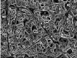
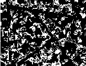
Let’s run this example using as input the image QB_Suburb.png provided in the directory Examples/Data.
We can easily segment the major structures by providing seeds in the appropriate locations and defining
values for the lower and upper thresholds. Figure 16.4 illustrates several examples of segmentation. The
parameters used are presented in Table 16.2.
|
|
|
|
|
| Structure | Seed Index | Lower | Upper | Output Image |
|
|
|
|
|
| Road | (110,38) | 50 | 100 | Second from left in Figure 16.4 |
|
|
|
|
|
| Shadow | (118,100) | 0 | 10 | Third from left in Figure 16.4 |
|
|
|
|
|
| Building | (169,146) | 220 | 255 | Fourth from left in Figure 16.4 |
|
|
|
|
|
| |
As with the ConnectedThresholdImageFilter, several seeds could be provided to the filter by using the
AddSeed() method. Compare the output of Figure 16.4 with those of Figure 16.1 produced by the
ConnectedThresholdImageFilter. You may want to play with the value of the neighborhood radius and see
how it affect the smoothness of the segmented object borders, the size of the segmented region and how
much that costs in computing time.
The source code for this example can be found in the file
Examples/Segmentation/ConfidenceConnected.cxx.
The following example illustrates the use of the itk::ConfidenceConnectedImageFilter . The
criterion used by the ConfidenceConnectedImageFilter is based on simple statistics of the current region.
First, the algorithm computes the mean and standard deviation of intensity values for all the pixels currently
included in the region. A user-provided factor is used to multiply the standard deviation and
define a range around the mean. Neighbor pixels whose intensity values fall inside the range
are accepted and included in the region. When no more neighbor pixels are found that satisfy
the criterion, the algorithm is considered to have finished its first iteration. At that point, the
mean and standard deviation of the intensity levels are recomputed using all the pixels currently
included in the region. This mean and standard deviation defines a new intensity range that is used
to visit current region neighbors and evaluate whether their intensity falls inside the range.
This iterative process is repeated until no more pixels are added or the maximum number of
iterations is reached. The following equation illustrates the inclusion criterion used by this
filter,
![I(X)∈ [m - fσ,m+ fσ]](SoftwareGuide296x.png) | (16.2) |
where m and σ are the mean and standard deviation of the region intensities, f is a factor defined by the
user, I() is the image and X is the position of the particular neighbor pixel being considered for inclusion in
the region.
Let’s look at the minimal code required to use this algorithm. First, the following header defining the
itk::ConfidenceConnectedImageFilter class must be included.
#include "itkConfidenceConnectedImageFilter.h"
Noise present in the image can reduce the capacity of this filter to grow large regions. When faced with
noisy images, it is usually convenient to pre-process the image by using an edge-preserving smoothing
filter. In this particular example we use the itk::CurvatureFlowImageFilter , hence we need to
include its header file.
#include "itkCurvatureFlowImageFilter.h"
We now define the image type using a pixel type and a particular dimension. In this case the float type is
used for the pixels due to the requirements of the smoothing filter.
typedef float InternalPixelType; const unsigned int Dimension = 2;
typedef otb::Image<InternalPixelType, Dimension> InternalImageType;
The smoothing filter type is instantiated using the image type as a template parameter.
typedef itk::CurvatureFlowImageFilter<InternalImageType, InternalImageType> CurvatureFlowImageFilterType;
Next the filter is created by invoking the New() method and assigning the result to a itk::SmartPointer
.
CurvatureFlowImageFilterType::Pointer smoothing = CurvatureFlowImageFilterType::New();
We now declare the type of the region growing filter. In this case it is the ConfidenceConnectedImageFilter.
typedef itk::ConfidenceConnectedImageFilter<InternalImageType, InternalImageType> ConnectedFilterType;
Then, we construct one filter of this class using the New() method.
ConnectedFilterType::Pointer confidenceConnected = ConnectedFilterType::New();
Now it is time to create a simple, linear pipeline. A file reader is added at the beginning of
the pipeline and a cast filter and writer are added at the end. The cast filter is required here to
convert float pixel types to integer types since only a few image file formats support float
types.
smoothing->SetInput(reader->GetOutput()); confidenceConnected->SetInput(smoothing->GetOutput());
caster->SetInput(confidenceConnected->GetOutput()); writer->SetInput(caster->GetOutput());
The CurvatureFlowImageFilter requires defining two parameters. The following are typical values.
However they may have to be adjusted depending on the amount of noise present in the input
image.
smoothing->SetNumberOfIterations(5); smoothing->SetTimeStep(0.125);
The ConfidenceConnectedImageFilter requires defining two parameters. First, the factor f that the defines
how large the range of intensities will be. Small values of the multiplier will restrict the inclusion of pixels
to those having very similar intensities to those in the current region. Larger values of the multiplier will
relax the accepting condition and will result in more generous growth of the region. Values that are too large
will cause the region to grow into neighboring regions that may actually belong to separate
structures.
confidenceConnected->SetMultiplier(2.5);
The number of iterations is specified based on the homogeneity of the intensities of the object to be
segmented. Highly homogeneous regions may only require a couple of iterations. Regions with
ramp effect, may require more iterations. In practice, it seems to be more important to carefully
select the multiplier factor than the number of iterations. However, keep in mind that there
is no reason to assume that this algorithm should converge to a stable region. It is possible
that by letting the algorithm run for more iterations the region will end up engulfing the entire
image.
confidenceConnected->SetNumberOfIterations(5);
The output of this filter is a binary image with zero-value pixels everywhere except on the extracted region.
The intensity value to be set inside the region is selected with the method SetReplaceValue()
confidenceConnected->SetReplaceValue(255);
The initialization of the algorithm requires the user to provide a seed point. It is convenient
to select this point to be placed in a typical region of the structure to be segmented. A small
neighborhood around the seed point will be used to compute the initial mean and standard deviation for
the inclusion criterion. The seed is passed in the form of a itk::Index to the SetSeed()
method.
confidenceConnected->SetSeed(index);
The size of the initial neighborhood around the seed is defined with the method
SetInitialNeighborhoodRadius(). The neighborhood will be defined as an N-dimensional
rectangular region with 2r+1 pixels on the side, where r is the value passed as initial neighborhood
radius.
confidenceConnected->SetInitialNeighborhoodRadius(2);
The invocation of the Update() method on the writer triggers the execution of the pipeline. It is
recommended to place update calls in a try/catch block in case errors occur and exceptions are
thrown.
try { writer->Update(); } catch (itk::ExceptionObject& excep) {
std::cerr << "Exception caught !" << std::endl; std::cerr << excep << std::endl; }
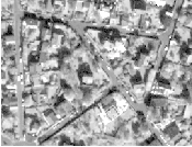
Let’s now run this example using as input the image QB_Suburb.png provided in the directory
Examples/Data. We can easily segment structures by providing seeds in the appropriate locations. For
example
|
|
|
|
|
| Structure | Seed Index | Lower | Upper | Output Image |
|
|
|
|
|
| Road | (110,38) | 50 | 100 | Second from left in Figure 16.1 |
|
|
|
|
|
| Shadow | (118,100) | 0 | 10 | Third from left in Figure 16.1 |
|
|
|
|
|
| Building | (169,146) | 220 | 255 | Fourth from left in Figure 16.1 |
|
|
|
|
|
| |
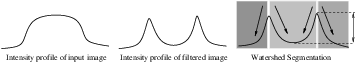
Watershed segmentation classifies pixels into regions using gradient descent on image features and analysis
of weak points along region boundaries. Imagine water raining onto a landscape topology and flowing with
gravity to collect in low basins. The size of those basins will grow with increasing amounts of precipitation
until they spill into one another, causing small basins to merge together into larger basins. Regions
(catchment basins) are formed by using local geometric structure to associate points in the image
domain with local extrema in some feature measurement such as curvature or gradient magnitude.
This technique is less sensitive to user-defined thresholds than classic region-growing methods,
and may be better suited for fusing different types of features from different data sets. The
watersheds technique is also more flexible in that it does not produce a single image segmentation,
but rather a hierarchy of segmentations from which a single region or set of regions can be
extracted a-priori, using a threshold, or interactively, with the help of a graphical user interface
[147, 148].
The strategy of watershed segmentation is to treat an image f as a height function, i.e., the surface formed
by graphing f as a function of its independent parameters,  ∈ U. The image f is often not the original input
data, but is derived from that data through some filtering, graded (or fuzzy) feature extraction, or fusion of
feature maps from different sources. The assumption is that higher values of f (or -f) indicate the presence
of boundaries in the original data. Watersheds may therefore be considered as a final or intermediate step in
a hybrid segmentation method, where the initial segmentation is the generation of the edge feature
map.
∈ U. The image f is often not the original input
data, but is derived from that data through some filtering, graded (or fuzzy) feature extraction, or fusion of
feature maps from different sources. The assumption is that higher values of f (or -f) indicate the presence
of boundaries in the original data. Watersheds may therefore be considered as a final or intermediate step in
a hybrid segmentation method, where the initial segmentation is the generation of the edge feature
map.
Gradient descent associates regions with local minima of f (clearly interior points) using the watersheds of
the graph of f, as in Figure 16.6.
That is, a segment consists of all points in U whose paths of steepest descent on the graph of f terminate at
the same minimum in f. Thus, there are as many segments in an image as there are minima in f. The
segment boundaries are “ridges” [80, 81, 44] in the graph of f. In the 1D case (U ⊂ℜ), the watershed
boundaries are the local maxima of f, and the results of the watershed segmentation is trivial. For
higher-dimensional image domains, the watershed boundaries are not simply local phenomena; they depend
on the shape of the entire watershed.
The drawback of watershed segmentation is that it produces a region for each local minimum—in practice
too many regions—and an over segmentation results. To alleviate this, we can establish a minimum
watershed depth. The watershed depth is the difference in height between the watershed minimum and the
lowest boundary point. In other words, it is the maximum depth of water a region could hold without
flowing into any of its neighbors. Thus, a watershed segmentation algorithm can sequentially combine
watersheds whose depths fall below the minimum until all of the watersheds are of sufficient depth. This
depth measurement can be combined with other saliency measurements, such as size. The result
is a segmentation containing regions whose boundaries and size are significant. Because the
merging process is sequential, it produces a hierarchy of regions, as shown in Figure 16.7.
Previous work has shown the benefit of a user-assisted approach that provides a graphical interface to this
hierarchy, so that a technician can quickly move from the small regions that lie within an area of interest to
the union of regions that correspond to the anatomical structure [148].
There are two different algorithms commonly used to implement watersheds: top-down and bottom-up. The
top-down, gradient descent strategy was chosen for ITK because we want to consider the output of
multi-scale differential operators, and the f in question will therefore have floating point values. The
bottom-up strategy starts with seeds at the local minima in the image and grows regions outward and
upward at discrete intensity levels (equivalent to a sequence of morphological operations and sometimes
called morphological watersheds [123].) This limits the accuracy by enforcing a set of discrete gray levels
on the image.
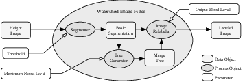
Figure 16.8 shows how the ITK image-to-image watersheds filter is constructed. The filter is actually a
collection of smaller filters that modularize the several steps of the algorithm in a mini-pipeline. The
segmenter object creates the initial segmentation via steepest descent from each pixel to local minima.
Shallow background regions are removed (flattened) before segmentation using a simple minimum value
threshold (this helps to minimize oversegmentation of the image). The initial segmentation is passed to a
second sub-filter that generates a hierarchy of basins to a user-specified maximum watershed depth. The
relabeler object at the end of the mini-pipeline uses the hierarchy and the initial segmentation to produce an
output image at any scale below the user-specified maximum. Data objects are cached in the mini-pipeline
so that changing watershed depths only requires a (fast) relabeling of the basic segmentation. The three
parameters that control the filter are shown in Figure 16.8 connected to their relevant processing
stages.
The source code for this example can be found in the file
Examples/Segmentation/WatershedSegmentation.cxx.
The following example illustrates how to preprocess and segment images using the
itk::WatershedImageFilter . Note that the care with which the data is preprocessed will greatly affect
the quality of your result. Typically, the best results are obtained by preprocessing the original image with
an edge-preserving diffusion filter, such as one of the anisotropic diffusion filters, or with the
bilateral image filter. As noted in Section 16.2.1, the height function used as input should be
created such that higher positive values correspond to object boundaries. A suitable height
function for many applications can be generated as the gradient magnitude of the image to be
segmented.
The itk::VectorGradientMagnitudeAnisotropicDiffusionImageFilter class is used to smooth
the image and the itk::VectorGradientMagnitudeImageFilter is used to generate the height
function. We begin by including all preprocessing filter header files and the header file for the
WatershedImageFilter. We use the vector versions of these filters because the input data is a color
image.
#include "itkVectorGradientAnisotropicDiffusionImageFilter.h"
#include "itkVectorGradientMagnitudeImageFilter.h" #include "itkWatershedImageFilter.h"
We now declare the image and pixel types to use for instantiation of the filters. All of these filters expect
real-valued pixel types in order to work properly. The preprocessing stages are done directly on the
vector-valued data and the segmentation is done using floating point scalar data. Images are converted from
RGB pixel type to numerical vector type using itk::VectorCastImageFilter . Please pay attention to
the fact that we are using itk::Image s since the itk::VectorGradientMagnitudeImageFilter has
some internal typedefs which make polymorfism impossible.
typedef itk::RGBPixel<unsigned char> RGBPixelType; typedef otb::Image<RGBPixelType, 2> RGBImageType;
typedef itk::Vector<float, 3> VectorPixelType; typedef itk::Image<VectorPixelType, 2> VectorImageType;
typedef itk::Image<unsigned long, 2> LabeledImageType;
typedef itk::Image<float, 2> ScalarImageType;
The various image processing filters are declared using the types created above and eventually used in the
pipeline.
typedef otb::ImageFileReader<RGBImageType> FileReaderType;
typedef itk::VectorCastImageFilter<RGBImageType, VectorImageType> CastFilterType;
typedef itk::VectorGradientAnisotropicDiffusionImageFilter<VectorImageType, VectorImageType>
DiffusionFilterType; typedef itk::VectorGradientMagnitudeImageFilter<VectorImageType, float,
ScalarImageType> GradientMagnitudeFilterType;
typedef itk::WatershedImageFilter<ScalarImageType> WatershedFilterType;
Next we instantiate the filters and set their parameters. The first step in the image processing pipeline is
diffusion of the color input image using an anisotropic diffusion filter. For this class of filters, the CFL
condition requires that the time step be no more than 0.25 for two-dimensional images, and no more than
0.125 for three-dimensional images. The number of iterations and the conductance term will be taken from
the command line. See Section 8.7.2 for more information on the ITK anisotropic diffusion
filters.
DiffusionFilterType::Pointer diffusion = DiffusionFilterType::New();
diffusion->SetNumberOfIterations(atoi(argv[4])); diffusion->SetConductanceParameter(atof(argv[3]));
diffusion->SetTimeStep(0.125); diffusion->SetUseImageSpacing(false);
The ITK gradient magnitude filter for vector-valued images can optionally take several parameters. Here we
allow only enabling or disabling of principal component analysis.
GradientMagnitudeFilterType::Pointer gradient = GradientMagnitudeFilterType::New();
gradient->SetUsePrincipleComponents(atoi(argv[7])); gradient->SetUseImageSpacingOff();
Finally we set up the watershed filter. There are two parameters. Level controls watershed depth, and
Threshold controls the lower thresholding of the input. Both parameters are set as a percentage (0.0 - 1.0)
of the maximum depth in the input image.
WatershedFilterType::Pointer watershed = WatershedFilterType::New();
watershed->SetLevel(atof(argv[6])); watershed->SetThreshold(atof(argv[5]));
The output of WatershedImageFilter is an image of unsigned long integer labels, where a label denotes
membership of a pixel in a particular segmented region. This format is not practical for visualization,
so for the purposes of this example, we will convert it to RGB pixels. RGB images have the
advantage that they can be saved as a simple png file and viewed using any standard image
viewer software. The itk::Functor::ScalarToRGBPixelFunctor class is a special function
object designed to hash a scalar value into an itk::RGBPixel . Plugging this functor into the
itk::UnaryFunctorImageFilter creates an image filter for that converts scalar images to RGB
images.
typedef itk::Functor::ScalarToRGBPixelFunctor<unsigned long> ColorMapFunctorType;
typedef itk::UnaryFunctorImageFilter<LabeledImageType, RGBImageType,
ColorMapFunctorType> ColorMapFilterType; ColorMapFilterType::Pointer colormapper = ColorMapFilterType::New();
The filters are connected into a single pipeline, with readers and writers at each end.
caster->SetInput(reader->GetOutput()); diffusion->SetInput(caster->GetOutput());
gradient->SetInput(diffusion->GetOutput()); watershed->SetInput(gradient->GetOutput());
colormapper->SetInput(watershed->GetOutput()); writer->SetInput(colormapper->GetOutput());
Tuning the filter parameters for any particular application is a process of trial and error. The threshold
parameter can be used to great effect in controlling oversegmentation of the image. Raising the threshold
will generally reduce computation time and produce output with fewer and larger regions. The trick in
tuning parameters is to consider the scale level of the objects that you are trying to segment in the image.
The best time/quality trade-off will be achieved when the image is smoothed and thresholded to eliminate
features just below the desired scale.
Figure 16.9 shows output from the example code. Note that a critical difference between the two
segmentations is the mode of the gradient magnitude calculation.
A note on the computational complexity of the watershed algorithm is warranted. Most of the complexity of
the ITK implementation lies in generating the hierarchy. Processing times for this stage are non-linear with
respect to the number of catchment basins in the initial segmentation. This means that the amount of
information contained in an image is more significant than the number of pixels in the image. A
very large, but very flat input take less time to segment than a very small, but very detailed
input.
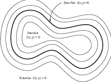
The paradigm of the level set is that it is a numerical method for tracking the evolution of contours and
surfaces. Instead of manipulating the contour directly, the contour is embedded as the zero level set of a
higher dimensional function called the level-set function, ψ(X,t). The level-set function is then evolved
under the control of a differential equation. At any time, the evolving contour can be obtained by extracting
the zero level-set Γ((X),t) = {ψ(X,t) = 0} from the output. The main advantages of using level sets is that
arbitrarily complex shapes can be modeled and topological changes such as merging and splitting are
handled implicitly.
Level sets can be used for image segmentation by using image-based features such as mean intensity,
gradient and edges in the governing differential equation. In a typical approach, a contour is initialized by a
user and is then evolved until it fits the form of an object in the image. Many different implementations and
variants of this basic concept have been published in the literature. An overview of the field has been made
by Sethian [124].
The following sections introduce practical examples of some of the level set segmentation methods
available in ITK. The remainder of this section describes features common to all of these filters except the
itk::FastMarchingImageFilter , which is derived from a different code framework. Understanding
these features will aid in using the filters more effectively.
Each filter makes use of a generic level-set equation to compute the update to the solution ψ of the partial
differential equation.
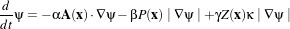 | (16.3) |
where A is an advection term, P is a propagation (expansion) term, and Z is a spatial modifier term for the
mean curvature κ. The scalar constants α, β, and γ weight the relative influence of each of the terms on the
movement of the interface. A segmentation filter may use all of these terms in its calculations, or it may
omit one or more terms. If a term is left out of the equation, then setting the corresponding scalar constant
weighting will have no effect.
All of the level-set based segmentation filters must operate with floating point precision to produce valid
results. The third, optional template parameter is the numerical type used for calculations and as the output
image pixel type. The numerical type is float by default, but can be changed to double for extra
precision. A user-defined, signed floating point type that defines all of the necessary arithmetic
operators and has sufficient precision is also a valid choice. You should not use types such as int
or unsigned char for the numerical parameter. If the input image pixel types do not match
the numerical type, those inputs will be cast to an image of appropriate type when the filter is
executed.
Most filters require two images as input, an initial model ψ(X,t = 0), and a feature image, which
is either the image you wish to segment or some preprocessed version. You must specify the
isovalue that represents the surface Γ in your initial model. The single image output of each filter
is the function ψ at the final time step. It is important to note that the contour representing
the surface Γ is the zero level-set of the output image, and not the isovalue you specified for
the initial model. To represent Γ using the original isovalue, simply add that value back to the
output.
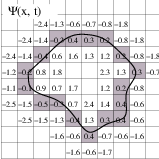
The solution Γ is calculated to subpixel precision. The best discrete approximation of the surface is
therefore the set of grid positions closest to the zero-crossings in the image, as shown in Figure 16.10. The
itk::ZeroCrossingImageFilter operates by finding exactly those grid positions and can be used to
extract the surface.
There are two important considerations when analyzing the processing time for any particular
level-set segmentation task: the surface area of the evolving interface and the total distance that the
surface must travel. Because the level-set equations are usually solved only at pixels near the
surface (fast marching methods are an exception), the time taken at each iteration depends on the
number of points on the surface. This means that as the surface grows, the solver will slow down
proportionally. Because the surface must evolve slowly to prevent numerical instabilities in the
solution, the distance the surface must travel in the image dictates the total number of iterations
required.
Some level-set techniques are relatively insensitive to initial conditions and are therefore suitable for region-growing
segmentation. Other techniques, such as the itk::LaplacianSegmentationLevelSetImageFilter ,
can easily become “stuck” on image features close to their initialization and should be used only when a
reasonable prior segmentation is available as the initialization. For best efficiency, your initial model of the
surface should be the best guess possible for the solution.
The source code for this example can be found in the file
Examples/Segmentation/FastMarchingImageFilter.cxx.
When the differential equation governing the level set evolution has a very simple form, a fast evolution
algorithm called fast marching can be used.
The following example illustrates the use of the itk::FastMarchingImageFilter . This filter
implements a fast marching solution to a simple level set evolution problem. In this example,
the speed term used in the differential equation is expected to be provided by the user in the
form of an image. This image is typically computed as a function of the gradient magnitude.
Several mappings are popular in the literature, for example, the negative exponential exp(-x)
and the reciprocal 1∕(1+x). In the current example we decided to use a Sigmoid function
since it offers a good deal of control parameters that can be customized to shape a nice speed
image.
The mapping should be done in such a way that the propagation speed of the front will be very low close to
high image gradients while it will move rather fast in low gradient areas. This arrangement will make the
contour propagate until it reaches the edges of anatomical structures in the image and then slow down
in front of those edges. The output of the FastMarchingImageFilter is a time-crossing map
that indicates, for each pixel, how much time it would take for the front to arrive at the pixel
location.
The application of a threshold in the output image is then equivalent to taking a snapshot of the
contour at a particular time during its evolution. It is expected that the contour will take a longer
time to cross over the edges of a particular structure. This should result in large changes on the
time-crossing map values close to the structure edges. Segmentation is performed with this filter by
locating a time range in which the contour was contained for a long time in a region of the image
space.
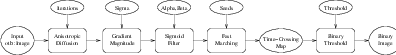
Figure 16.11 shows the major components involved in the application of the FastMarchingImageFilter to a segmentation
task. It involves an initial stage of smoothing using the itk::CurvatureAnisotropicDiffusionImageFilter
. The smoothed image is passed as the input to the itk::GradientMagnitudeRecursiveGaussianImageFilter
and then to the itk::SigmoidImageFilter . Finally, the output of the FastMarchingImageFilter is passed
to a itk::BinaryThresholdImageFilter in order to produce a binary mask representing the segmented
object.
The code in the following example illustrates the typical setup of a pipeline for performing
segmentation with fast marching. First, the input image is smoothed using an edge-preserving filter.
Then the magnitude of its gradient is computed and passed to a sigmoid filter. The result of the
sigmoid filter is the image potential that will be used to affect the speed term of the differential
equation.
Let’s start by including the following headers. First we include the header of the
CurvatureAnisotropicDiffusionImageFilter that will be used for removing noise from the input
image.
#include "itkCurvatureAnisotropicDiffusionImageFilter.h"
The headers of the GradientMagnitudeRecursiveGaussianImageFilter and SigmoidImageFilter are included
below. Together, these two filters will produce the image potential for regulating the speed term in the
differential equation describing the evolution of the level set.
#include "itkGradientMagnitudeRecursiveGaussianImageFilter.h" #include "itkSigmoidImageFilter.h"
Of course, we will need the otb::Image class and the FastMarchingImageFilter class. Hence we include
their headers.
#include "otbImage.h" #include "itkFastMarchingImageFilter.h"
The time-crossing map resulting from the FastMarchingImageFilter will be thresholded using the
BinaryThresholdImageFilter. We include its header here.
#include "itkBinaryThresholdImageFilter.h"
Reading and writing images will be done with the otb::ImageFileReader and otb::ImageFileWriter
.
#include "otbImageFileReader.h" #include "otbImageFileWriter.h"
We now define the image type using a pixel type and a particular dimension. In this case the float type is
used for the pixels due to the requirements of the smoothing filter.
typedef float InternalPixelType; const unsigned int Dimension = 2;
typedef otb::Image<InternalPixelType, Dimension> InternalImageType;
The output image, on the other hand, is declared to be binary.
typedef unsigned char OutputPixelType;
typedef otb::Image<OutputPixelType, Dimension> OutputImageType;
The type of the BinaryThresholdImageFilter filter is instantiated below using the internal image type and
the output image type.
typedef itk::BinaryThresholdImageFilter<InternalImageType, OutputImageType>
ThresholdingFilterType; ThresholdingFilterType::Pointer thresholder = ThresholdingFilterType::New();
The upper threshold passed to the BinaryThresholdImageFilter will define the time snapshot that we are
taking from the time-crossing map.
thresholder->SetLowerThreshold(0.0); thresholder->SetUpperThreshold(timeThreshold);
thresholder->SetOutsideValue(0); thresholder->SetInsideValue(255);
We instantiate reader and writer types in the following lines.
typedef otb::ImageFileReader<InternalImageType> ReaderType;
typedef otb::ImageFileWriter<OutputImageType> WriterType;
The CurvatureAnisotropicDiffusionImageFilter type is instantiated using the internal image
type.
typedef itk::CurvatureAnisotropicDiffusionImageFilter< InternalImageType,
InternalImageType> SmoothingFilterType;
Then, the filter is created by invoking the New() method and assigning the result to a itk::SmartPointer
.
SmoothingFilterType::Pointer smoothing = SmoothingFilterType::New();
The types of the GradientMagnitudeRecursiveGaussianImageFilter and SigmoidImageFilter are instantiated
using the internal image type.
typedef itk::GradientMagnitudeRecursiveGaussianImageFilter< InternalImageType,
InternalImageType> GradientFilterType; typedef itk::SigmoidImageFilter<
InternalImageType, InternalImageType> SigmoidFilterType;
The corresponding filter objects are instantiated with the New() method.
GradientFilterType::Pointer gradientMagnitude = GradientFilterType::New();
SigmoidFilterType::Pointer sigmoid = SigmoidFilterType::New();
The minimum and maximum values of the SigmoidImageFilter output are defined with the methods
SetOutputMinimum() and SetOutputMaximum(). In our case, we want these two values to be 0.0 and 1.0
respectively in order to get a nice speed image to feed to the FastMarchingImageFilter.
sigmoid->SetOutputMinimum(0.0); sigmoid->SetOutputMaximum(1.0);
We now declare the type of the FastMarchingImageFilter.
typedef itk::FastMarchingImageFilter<InternalImageType, InternalImageType> FastMarchingFilterType;
Then, we construct one filter of this class using the New() method.
FastMarchingFilterType::Pointer fastMarching = FastMarchingFilterType::New();
The filters are now connected in a pipeline shown in Figure 16.11 using the following lines.
smoothing->SetInput(reader->GetOutput()); gradientMagnitude->SetInput(smoothing->GetOutput());
sigmoid->SetInput(gradientMagnitude->GetOutput()); fastMarching->SetInput(sigmoid->GetOutput());
thresholder->SetInput(fastMarching->GetOutput()); writer->SetInput(thresholder->GetOutput());
The CurvatureAnisotropicDiffusionImageFilter class requires a couple of parameters to be defined. The
following are typical values. However they may have to be adjusted depending on the amount of noise
present in the input image.
smoothing->SetTimeStep(0.125); smoothing->SetNumberOfIterations(10); smoothing->SetConductanceParameter(2.0);
The GradientMagnitudeRecursiveGaussianImageFilter performs the equivalent of a convolution with a
Gaussian kernel followed by a derivative operator. The sigma of this Gaussian can be used to control the
range of influence of the image edges.
gradientMagnitude->SetSigma(sigma);
The SigmoidImageFilter class requires two parameters to define the linear transformation to be applied to
the sigmoid argument. These parameters are passed using the SetAlpha() and SetBeta() methods. In the
context of this example, the parameters are used to intensify the differences between regions of low and
high values in the speed image. In an ideal case, the speed value should be 1.0 in the homogeneous regions
and the value should decay rapidly to 0.0 around the edges of structures. The heuristic for finding the values
is the following. From the gradient magnitude image, let’s call K1 the minimum value along the contour of
the structure to be segmented. Then, let’s call K2 an average value of the gradient magnitude in the
middle of the structure. These two values indicate the dynamic range that we want to map to
the interval [0 : 1] in the speed image. We want the sigmoid to map K1 to 0.0 and K2 to 1.0.
Given that K1 is expected to be higher than K2 and we want to map those values to 0.0 and 1.0
respectively, we want to select a negative value for alpha so that the sigmoid function will also do an
inverse intensity mapping. This mapping will produce a speed image such that the level set
will march rapidly on the homogeneous region and will definitely stop on the contour. The
suggested value for beta is (K1+K2)∕2 while the suggested value for alpha is (K2-K1)∕6, which
must be a negative number. In our simple example the values are provided by the user from the
command line arguments. The user can estimate these values by observing the gradient magnitude
image.
sigmoid->SetAlpha(alpha); sigmoid->SetBeta(beta);
The FastMarchingImageFilter requires the user to provide a seed point from which the contour will expand.
The user can actually pass not only one seed point but a set of them. A good set of seed points increases the
chances of segmenting a complex object without missing parts. The use of multiple seeds also helps to
reduce the amount of time needed by the front to visit a whole object and hence reduces the risk of leaks on
the edges of regions visited earlier. For example, when segmenting an elongated object, it is undesirable to
place a single seed at one extreme of the object since the front will need a long time to propagate to
the other end of the object. Placing several seeds along the axis of the object will probably
be the best strategy to ensure that the entire object is captured early in the expansion of the
front. One of the important properties of level sets is their natural ability to fuse several fronts
implicitly without any extra bookkeeping. The use of multiple seeds takes good advantage of this
property.
The seeds are passed stored in a container. The type of this container is defined as NodeContainer among
the FastMarchingImageFilter traits.
typedef FastMarchingFilterType::NodeContainer NodeContainer;
typedef FastMarchingFilterType::NodeType NodeType; NodeContainer::Pointer seeds = NodeContainer::New();
Nodes are created as stack variables and initialized with a value and an itk::Index position.
NodeType node; const double seedValue = 0.0; node.SetValue(seedValue); node.SetIndex(seedPosition);
The list of nodes is initialized and then every node is inserted using the InsertElement().
seeds->Initialize(); seeds->InsertElement(0, node);
The set of seed nodes is now passed to the FastMarchingImageFilter with the method SetTrialPoints().
fastMarching->SetTrialPoints(seeds);
The FastMarchingImageFilter requires the user to specify the size of the image to be produced as output.
This is done using the SetOutputSize(). Note that the size is obtained here from the output image of the
smoothing filter. The size of this image is valid only after the Update() methods of this filter has been
called directly or indirectly.
fastMarching->SetOutputSize( reader->GetOutput()->GetBufferedRegion().GetSize());
Since the front representing the contour will propagate continuously over time, it is desirable to stop the
process once a certain time has been reached. This allows us to save computation time under the assumption
that the region of interest has already been computed. The value for stopping the process is defined with the
method SetStoppingValue(). In principle, the stopping value should be a little bit higher than the
threshold value.
fastMarching->SetStoppingValue(stoppingTime);
The invocation of the Update() method on the writer triggers the execution of the pipeline.
As usual, the call is placed in a try/catch block should any errors occur or exceptions be
thrown.
try { writer->Update(); } catch (itk::ExceptionObject& excep) {
std::cerr << "Exception caught !" << std::endl; std::cerr << excep << std::endl; }
Now let’s run this example using the input image QB_Suburb.png provided in the directory
Examples/Data. We can easily segment structures by providing seeds in the appropriate locations. The
following table presents the parameters used for some structures.
|
|
|
|
|
|
|
|
| Structure | Seed Index | σ | α | β | Threshold | Output Image from left |
|
|
|
|
|
|
|
|
| Road | (91,176) | 0.5 | -0.5 | 3.0 | 100 | First |
|
|
|
|
|
|
|
|
| Shadow | (118,100) | 1.0 | -0.5 | 3.0 | 100 | Second |
|
|
|
|
|
|
|
|
| Building | (145,21) | 0.5 | -0.5 | 3.0 | 100 | Third |
|
|
|
|
|
|
|
|
| |
Table 16.4: Parameters used for segmenting some structures shown in Figure 16.13 using the filter
FastMarchingImageFilter. All of them used a stopping value of 100.
Figure 16.12 presents the intermediate outputs of the pipeline illustrated in Figure 16.11. They are from
left to right: the output of the anisotropic diffusion filter, the gradient magnitude of the smoothed image
and the sigmoid of the gradient magnitude which is finally used as the speed image for the
FastMarchingImageFilter.
The following classes provide similar functionality:
See the ITK Software Guide for examples of the use of these classes.