This chapter introduces the most commonly used filters found in OTB. Most of these filters are intended to process images. They will accept one or more images as input and will produce one or more images as output. OTB is based ITK’s data pipeline architecture in which the output of one filter is passed as input to another filter. (See Section 3.5 on page 61 for more information.)
The thresholding operation is used to change or identify pixel values based on specifying one or more values (called the threshold value). The following sections describe how to perform thresholding operations using OTB.
The source code for this example can be found in the file
Examples/Filtering/BinaryThresholdImageFilter.cxx.
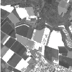
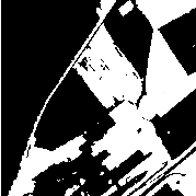
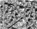
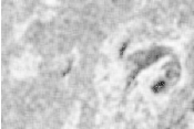
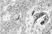
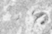
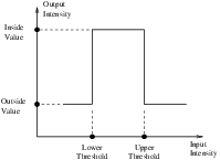
This example illustrates the use of the binary threshold image filter. This filter is used to transform an image into a binary image by changing the pixel values according to the rule illustrated in Figure ??. The user defines two thresholds—Upper and Lower—and two intensity values—Inside and Outside. For each pixel in the input image, the value of the pixel is compared with the lower and upper thresholds. If the pixel value is inside the range defined by [Lower,Upper] the output pixel is assigned the InsideValue. Otherwise the output pixels are assigned to the OutsideValue. Thresholding is commonly applied as the last operation of a segmentation pipeline.
The first step required to use the itk::BinaryThresholdImageFilter is to include its header file.
The next step is to decide which pixel types to use for the input and output images.
The input and output image types are now defined using their respective pixel types and dimensions.
The filter type can be instantiated using the input and output image types defined above.
An otb::ImageFileReader class is also instantiated in order to read image data from a file. (See Section 6 on page 149 for more information about reading and writing data.)
An otb::ImageFileWriter is instantiated in order to write the output image to a file.
Both the filter and the reader are created by invoking their New() methods and assigning the result to itk::SmartPointer s.
The image obtained with the reader is passed as input to the BinaryThresholdImageFilter.
The method SetOutsideValue() defines the intensity value to be assigned to those pixels whose intensities are outside the range defined by the lower and upper thresholds. The method SetInsideValue() defines the intensity value to be assigned to pixels with intensities falling inside the threshold range.
The methods SetLowerThreshold() and SetUpperThreshold() define the range of the input image intensities that will be transformed into the InsideValue. Note that the lower and upper thresholds are values of the type of the input image pixels, while the inside and outside values are of the type of the output image pixels.
The execution of the filter is triggered by invoking the Update() method. If the filter’s output has been passed as input to subsequent filters, the Update() call on any posterior filters in the pipeline will indirectly trigger the update of this filter.
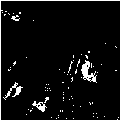
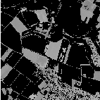
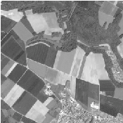
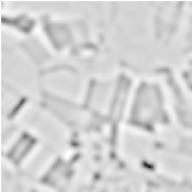
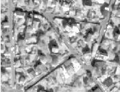
Figure 8.1 illustrates the effect of this filter on a ROI of a Spot 5 image of an agricultural area. This figure shows the limitations of this filter for performing segmentation by itself. These limitations are particularly noticeable in noisy images and in images lacking spatial uniformity.
The following classes provide similar functionality:
The source code for this example can be found in the file
Examples/Filtering/ThresholdImageFilter.cxx.
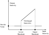
This example illustrates the use of the itk::ThresholdImageFilter . This filter can be used to transform the intensity levels of an image in three different ways.
The following methods choose among the three operating modes of the filter.
The first step required to use this filter is to include its header file.
Then we must decide what pixel type to use for the image. This filter is templated over a single image type because the algorithm only modifies pixel values outside the specified range, passing the rest through unchanged.
The image is defined using the pixel type and the dimension.
The filter can be instantiated using the image type defined above.
An otb::ImageFileReader class is also instantiated in order to read image data from a file.
An otb::ImageFileWriter is instantiated in order to write the output image to a file.
Both the filter and the reader are created by invoking their New() methods and assigning the result to SmartPointers.
The image obtained with the reader is passed as input to the itk::ThresholdImageFilter .
The method SetOutsideValue() defines the intensity value to be assigned to those pixels whose intensities are outside the range defined by the lower and upper thresholds.
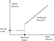
The method ThresholdBelow() defines the intensity value below which pixels of the input image will be changed to the OutsideValue.
The filter is executed by invoking the Update() method. If the filter is part of a larger image processing pipeline, calling Update() on a downstream filter will also trigger update of this filter.
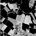
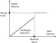
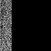
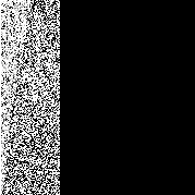
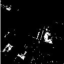
The output of this example is shown in Figure 8.2. The second operating mode of the filter is now enabled by calling the method ThresholdAbove().
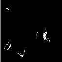
Updating the filter with this new setting produces the output shown in Figure 8.3. The third operating mode of the filter is enabled by calling ThresholdOutside().
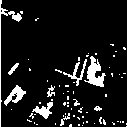
The output of this third, “band-pass” thresholding mode is shown in Figure 8.4.
The examples in this section also illustrate the limitations of the thresholding filter for performing segmentation by itself. These limitations are particularly noticeable in noisy images and in images lacking spatial uniformity.
The following classes provide similar functionality:
The source code for this example can be found in the file
Examples/FeatureExtraction/ThresholdToPointSetExample.cxx.
Sometimes, it may be more valuable not to get an image from the threshold step but rather a list of coordinates. This can be done with the otb::ThresholdImageToPointSetFilter .
The following example illustrates the use of the otb::ThresholdImageToPointSetFilter which provide a list of points within given thresholds. Points set are described in section 5.2 on page 125.
The first step required to use this filter is to include the header
The next step is to decide which pixel types to use for the input image and the Point Set as well as their dimension.
A reader is instantiated to read the input image
We get the parameters from the command line for the threshold filter. The lower and upper thresholds parameters are similar to those of the itk::BinaryThresholdImageFilter (see Section 8.1.1 on page 201 for more information).
Then we create the ThresholdImageToPointSetFilter and we pass the parameters.
To manipulate and display the result of this filter, we manually instantiate a point set and we call the Update() method on the threshold filter to trigger the pipeline execution.
After this step, the pointSet variable contains the point set.
To display each point, we create an iterator on the list of points, which is accessible through the method GetPoints() of the PointSet.
A while loop enable us to through the list a display the coordinate of each point.
OTB and ITK provide a lot of filters allowing to perform basic operations on image layers (thresholding, ratio, layers combinations...). It allows to create a processing chain defining at each step operations and to combine them in the data pipeline. But the library offers also the possibility to perform more generic complex mathematical operation on images in a single filter: the otb::BandMathImageFilter and more recently the otb::BandMathImageFilterX .
The source code for this example can be found in the file
Examples/BasicFilters/BandMathFilterExample.cxx.
This filter is based on the mathematical parser library muParser. The built in functions and operators list is available at: http://muparser.sourceforge.net/mup_features.html.
In order to use this filter, at least one input image should be set. An associated variable name can be specified or not by using the corresponding SetNthInput method. For the nth input image, if no associated variable name has been specified, a default variable name is given by concatenating the letter ”b” (for band) and the corresponding input index.
The next step is to set the expression according to the variable names. For example, in the default case with three input images the following expression is valid : ”(b1+b2)*b3”.
We start by including the required header file. The aim of this example is to compute the Normalized Difference Vegetation Index (NDVI) from a multispectral image and then apply a threshold to this index to extract areas containing a dense vegetation canopy.
We start by the classical typedefs needed for reading and writing the images. The otb::BandMathImageFilter class works with otb::Image as input, so we need to define additional filters to extract each layer of the multispectral image.
We can now define the type for the filter:
We instantiate the filter, the reader, and the writer:
We now need to extract each band from the input otb::VectorImage , it illustrates the use of the otb::VectorImageToImageList . Each extracted layer is an input to the otb::BandMathImageFilter :
Now we can define the mathematical expression to perform on the layers (b1, b2, b3, b4). The filter takes advantage of the parsing capabilities of the muParser library and allows setting the expression as on a digital calculator.
The expression below returns 255 if the ratio (NIR-RED)∕(NIR+RED) is greater than 0.4 and 0 if not.
We can now plug the pipeline and run it.
The muParser library also provides the possibility to extend existing built-in functions. For example, you can use the OTB expression ”ndvi(b3, b4)” with the filter. In this instance, the mathematical expression would be if(ndvi(b3,b4) > 0.4, 255, 0), which would return the same result.
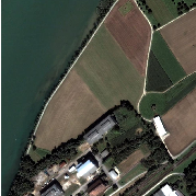
Figure 8.5 shows the result of the threshold applied to the NDVI index of a Quickbird image.
A new version of the BandMath filter is now available; among the new functionalities, variables representing multi-band pixels were introduced, as well as variables representing neighborhoods of pixels. The class name is otb::BandMathImageFilterX .
The source code for this example can be found in the file
Examples/BasicFilters/BandMathXImageFilterExample.cxx.
This filter is based on the mathematical parser library muParserX. The built in functions and operators list is available at: http://articles.beltoforion.de/article.php?a=muparserx.
In order to use this filter, at least one input image is to be set. An associated variable name can be specified or not by using the corresponding SetNthInput method. For the jth (j=1..T) input image, if no associated variable name has been specified, a default variable name is given by concatenating the prefix ”im” with the corresponding input index plus one (for instance, im1 is related to the first input). If the jth input image is multidimensional, then the variable imj represents a vector whose components are related to its bands. In order to access the kth band, the variable observes the following pattern : imjbk.
We start by including the needed header files.
Then, we set the classical typedefs needed for reading and writing the images. The otb::BandMathXImageFilter class works with otb::VectorImage .
We can now define the type for the filter:
We instantiate the filter, the reader, and the writer:
The reader and the writer are parametrized with usual settings:
The aim of this example is to compute a simple high-pass filter. For that purpose, we are going to perform the difference between the original signal and its averaged version. The definition of the expression that follows is only suitable for a 4-band image. So first, we must check this requirement:
Now, we can define the expression. The variable im1 represents a pixel (made of 4 components) of the input image. The variable im1b1N5x5 represents a neighborhood of size 5x5 around this pixel (and so on for each band). The last element we need is the operator ’mean’. By setting its inputs with four neigborhoods, we tell this operator to process the four related bands. As output, it will produce a vector of four components; this is consistent with the fact that we wish to perform a difference with im1.
Thus, the expression is as follows:
Note that the importance of the averaging is driven by the names of the neighborhood variables. Last thing we have to do, is to set the pipeline:
Figure 8.6 shows the result of our high-pass filter.
Now let’s see a little bit more complex example. The aim now is to give the central pixel a higher weight. Moreover : - we wish to use smaller neighborhoods - we wish to drop the 4th band - we wish to add a given number to each band.
First, we instantiate new filters to later make a proper pipeline:
We define a new kernel (rows are separated by semi-colons, whereas their elements are separated by commas):
We then define a new constant:
We now set the expression (note the use of ’dotpr’ operator, as well as the ’bands’ operator which is used as a band selector):
It is possible to export these definitions to a txt file (they will be reusable later thanks to the method ImportContext):
And finally, we set the pipeline:
Figure 8.7 shows the result of the second filter.
Finally, it is strongly recommended to take a look at the cookbook, where additional information and examples can be found (http://www.orfeo-toolbox.org/packages/OTBCookBook.pdf).
Computation of gradients is a fairly common operation in image processing. The term “gradient” may refer in some contexts to the gradient vectors and in others to the magnitude of the gradient vectors. ITK filters attempt to reduce this ambiguity by including the magnitude term when appropriate. ITK provides filters for computing both the image of gradient vectors and the image of magnitudes.
The source code for this example can be found in the file
Examples/Filtering/GradientMagnitudeImageFilter.cxx.
The magnitude of the image gradient is extensively used in image analysis, mainly to help in the determination of object contours and the separation of homogeneous regions. The itk::GradientMagnitudeImageFilter computes the magnitude of the image gradient at each pixel location using a simple finite differences approach. For example, in the case of 2D the computation is equivalent to convolving the image with masks of type
then adding the sum of their squares and computing the square root of the sum.
This filter will work on images of any dimension thanks to the internal use of itk::NeighborhoodIterator and itk::NeighborhoodOperator .
The first step required to use this filter is to include its header file.
Types should be chosen for the pixels of the input and output images.
The input and output image types can be defined using the pixel types.
The type of the gradient magnitude filter is defined by the input image and the output image types.
A filter object is created by invoking the New() method and assigning the result to a itk::SmartPointer .
The input image can be obtained from the output of another filter. Here, the source is an image reader.
Finally, the filter is executed by invoking the Update() method.
If the output of this filter has been connected to other filters in a pipeline, updating any of the downstream filters will also trigger an update of this filter. For example, the gradient magnitude filter may be connected to an image writer.
Figure 8.8 illustrates the effect of the gradient magnitude. The figure shows the sensitivity of this filter to noisy data.
Attention should be paid to the image type chosen to represent the output image since the dynamic range of the gradient magnitude image is usually smaller than the dynamic range of the input image. As always, there are exceptions to this rule, for example, images of man-made objects that contain high contrast objects.
This filter does not apply any smoothing to the image before computing the gradients. The results can therefore be very sensitive to noise and may not be best choice for scale space analysis.
The source code for this example can be found in the file
Examples/Filtering/GradientMagnitudeRecursiveGaussianImageFilter.cxx.
Differentiation is an ill-defined operation over digital data. In practice it is convenient to define a scale in which the differentiation should be performed. This is usually done by preprocessing the data with a smoothing filter. It has been shown that a Gaussian kernel is the most convenient choice for performing such smoothing. By choosing a particular value for the standard deviation (σ) of the Gaussian, an associated scale is selected that ignores high frequency content, commonly considered image noise.
The itk::GradientMagnitudeRecursiveGaussianImageFilter computes the magnitude of the image gradient at each pixel location. The computational process is equivalent to first smoothing the image by convolving it with a Gaussian kernel and then applying a differential operator. The user selects the value of σ.
Internally this is done by applying an IIR 1 filter that approximates a convolution with the derivative of the Gaussian kernel. Traditional convolution will produce a more accurate result, but the IIR approach is much faster, especially using large σs [36, 37].
GradientMagnitudeRecursiveGaussianImageFilter will work on images of any dimension by taking advantage of the natural separability of the Gaussian kernel and its derivatives.
The first step required to use this filter is to include its header file.
Types should be instantiated based on the pixels of the input and output images.
With them, the input and output image types can be instantiated.
The filter type is now instantiated using both the input image and the output image types.
A filter object is created by invoking the New() method and assigning the result to a itk::SmartPointer .
The input image can be obtained from the output of another filter. Here, an image reader is used as source.
The standard deviation of the Gaussian smoothing kernel is now set.
Finally the filter is executed by invoking the Update() method.
If connected to other filters in a pipeline, this filter will automatically update when any downstream filters are updated. For example, we may connect this gradient magnitude filter to an image file writer and then update the writer.
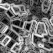
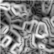
Figure 8.9 illustrates the effect of this filter using σ values of 3 (left) and 5 (right). The figure shows how the sensitivity to noise can be regulated by selecting an appropriate σ. This type of scale-tunable filter is suitable for performing scale-space analysis.
Attention should be paid to the image type chosen to represent the output image since the dynamic range of the gradient magnitude image is usually smaller than the dynamic range of the input image.
The source code for this example can be found in the file
Examples/Filtering/DerivativeImageFilter.cxx.
The itk::DerivativeImageFilter is used for computing the partial derivative of an image, the derivative of an image along a particular axial direction.
The header file corresponding to this filter should be included first.
Next, the pixel types for the input and output images must be defined and, with them, the image types can be instantiated. Note that it is important to select a signed type for the image, since the values of the derivatives will be positive as well as negative.
Using the image types, it is now possible to define the filter type and create the filter object.
The order of the derivative is selected with the SetOrder() method. The direction along which the derivative will be computed is selected with the SetDirection() method.
The input to the filter can be taken from any other filter, for example a reader. The output can be passed down the pipeline to other filters, for example, a writer. An update call on any downstream filter will trigger the execution of the derivative filter.
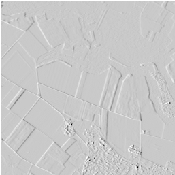
Figure 8.10 illustrates the effect of the DerivativeImageFilter. The derivative is taken along the x direction. The sensitivity to noise in the image is evident from this result.
The source code for this example can be found in the file
Examples/Filtering/LaplacianRecursiveGaussianImageFilter1.cxx.
This example illustrates how to use the itk::RecursiveGaussianImageFilter for computing the Laplacian of an image.
The first step required to use this filter is to include its header file.
Types should be selected on the desired input and output pixel types.
The input and output image types are instantiated using the pixel types.
The filter type is now instantiated using both the input image and the output image types.
This filter applies the approximation of the convolution along a single dimension. It is therefore necessary to concatenate several of these filters to produce smoothing in all directions. In this example, we create a pair of filters since we are processing a 2D image. The filters are created by invoking the New() method and assigning the result to a itk::SmartPointer .
We need two filters for computing the X component of the Laplacian and two other filters for computing the Y component.
Since each one of the newly created filters has the potential to perform filtering along any dimension, we have to restrict each one to a particular direction. This is done with the SetDirection() method.
The itk::RecursiveGaussianImageFilter can approximate the convolution with the Gaussian or with its first and second derivatives. We select one of these options by using the SetOrder() method. Note that the argument is an enum whose values can be ZeroOrder, FirstOrder and SecondOrder. For example, to compute the x partial derivative we should select FirstOrder for x and ZeroOrder for y. Here we want only to smooth in x and y, so we select ZeroOrder in both directions.
There are two typical ways of normalizing Gaussians depending on their application. For scale-space analysis it is desirable to use a normalization that will preserve the maximum value of the input. This normalization is represented by the following equation.
 | (8.1) |
In applications that use the Gaussian as a solution of the diffusion equation it is desirable to use a normalization that preserve the integral of the signal. This last approach can be seen as a conservation of mass principle. This is represented by the following equation.
 | (8.2) |
The itk::RecursiveGaussianImageFilter has a boolean flag that allows users to select between these two normalization options. Selection is done with the method SetNormalizeAcrossScale(). Enable this flag to analyzing an image across scale-space. In the current example, this setting has no impact because we are actually renormalizing the output to the dynamic range of the reader, so we simply disable the flag.
The input image can be obtained from the output of another filter. Here, an image reader is used as the source. The image is passed to the x filter and then to the y filter. The reason for keeping these two filters separate is that it is usual in scale-space applications to compute not only the smoothing but also combinations of derivatives at different orders and smoothing. Some factorization is possible when separate filters are used to generate the intermediate results. Here this capability is less interesting, though, since we only want to smooth the image in all directions.
It is now time to select the σ of the Gaussian used to smooth the data. Note that σ must be passed to both filters and that sigma is considered to be in the units of the image spacing. That is, at the moment of applying the smoothing process, the filter will take into account the spacing values defined in the image.
Finally the two components of the Laplacian should be added together. The itk::AddImageFilter is used for this purpose.
The filters are triggered by invoking Update() on the Add filter at the end of the pipeline.
The resulting image could be saved to a file using the otb::ImageFileWriter class.
Figure 8.11 illustrates the effect of this filter using σ values of 3 (left) and 5 (right). The figure shows how the attenuation of noise can be regulated by selecting the appropriate standard deviation. This type of scale-tunable filter is suitable for performing scale-space analysis.
The source code for this example can be found in the file
Examples/Filtering/LaplacianRecursiveGaussianImageFilter2.cxx.
The previous exampled showed how to use the itk::RecursiveGaussianImageFilter for computing the equivalent of a Laplacian of an image after smoothing with a Gaussian. The elements used in this previous example have been packaged together in the itk::LaplacianRecursiveGaussianImageFilter in order to simplify its usage. This current example shows how to use this convenience filter for achieving the same results as the previous example.
The first step required to use this filter is to include its header file.
Types should be selected on the desired input and output pixel types.
The input and output image types are instantiated using the pixel types.
The filter type is now instantiated using both the input image and the output image types.
This filter packages all the components illustrated in the previous example. The filter is created by invoking the New() method and assigning the result to a itk::SmartPointer .
The option for normalizing across scale space can also be selected in this filter.
The input image can be obtained from the output of another filter. Here, an image reader is used as the source.
It is now time to select the σ of the Gaussian used to smooth the data. Note that σ must be passed to both filters and that sigma is considered to be in the units of the image spacing. That is, at the moment of applying the smoothing process, the filter will take into account the spacing values defined in the image.
Finally the pipeline is executed by invoking the Update() method.
Figure 8.12 illustrates the effect of this filter using σ values of 3 (left) and 5 (right). The figure shows how the attenuation of noise can be regulated by selecting the appropriate standard deviation. This type of scale-tunable filter is suitable for performing scale-space analysis.
The source code for this example can be found in the file
Examples/Filtering/CannyEdgeDetectionImageFilter.cxx.
This example introduces the use of the itk::CannyEdgeDetectionImageFilter . This filter is widely used for edge detection since it is the optimal solution satisfying the constraints of good sensitivity, localization and noise robustness.
The first step required for using this filter is to include its header file
As the Canny filter works with real values, we can instantiated the reader using an image with pixels as double. This does not imply anything on the real image coding format which will be cast into double.
The itk::CannyEdgeDetectionImageFilter is instantiated using the float image type.
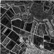
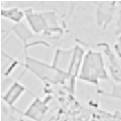
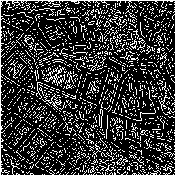
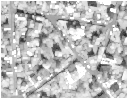
Figure 8.13 illustrates the effect of this filter on a ROI of a Spot 5 image of an agricultural area.
The source code for this example can be found in the file
Examples/FeatureExtraction/TouziEdgeDetectorExample.cxx.
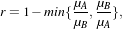
This example illustrates the use of the otb::TouziEdgeDetectorImageFilter . This filter belongs to the family of the fixed false alarm rate edge detectors but it is appropriate for SAR images, where the speckle noise is considered as multiplicative. By analogy with the classical gradient-based edge detectors which are suited to the additive noise case, this filter computes a ratio of local means in both sides of the edge [129]. In order to have a normalized response, the following computation is performed :
 | (8.3) |
where μA and μB are the local means computed at both sides of the edge. In order to detect edges with any orientation, r is computed for the 4 principal directions and the maximum response is kept.
The first step required to use this filter is to include its header file.
Then we must decide what pixel type to use for the image. We choose to make all computations with floating point precision and rescale the results between 0 and 255 in order to export PNG images.
The images are defined using the pixel type and the dimension.
The filter can be instantiated using the image types defined above.
An otb::ImageFileReader class is also instantiated in order to read image data from a file.
An otb::ImageFileWriter is instantiated in order to write the output image to a file.
The intensity rescaling of the results will be carried out by the itk::RescaleIntensityImageFilter which is templated by the input and output image types.
Both the filter and the reader are created by invoking their New() methods and assigning the result to SmartPointers.
The same is done for the rescaler and the writer.
The itk::RescaleIntensityImageFilter needs to know which is the minimu and maximum values of the output generated image. Those can be chosen in a generic way by using the NumericTraits functions, since they are templated over the pixel type.
The image obtained with the reader is passed as input to the otb::TouziEdgeDetectorImageFilter . The pipeline is built as follows.
The method SetRadius() defines the size of the window to be used for the computation of the local means.
The filter is executed by invoking the Update() method. If the filter is part of a larger image processing pipeline, calling Update() on a downstream filter will also trigger update of this filter.
We can also obtain the direction of the edges by invoking the GetOutputDirection() method.
Figure 8.14 shows the result of applying the Touzi edge detector filter to a SAR image.


The concept of locality is frequently encountered in image processing in the form of filters that compute every output pixel using information from a small region in the neighborhood of the input pixel. The classical form of these filters are the 3×3 filters in 2D images. Convolution masks based on these neighborhoods can perform diverse tasks ranging from noise reduction, to differential operations, to mathematical morphology.
The Insight toolkit implements an elegant approach to neighborhood-based image filtering. The input image is processed using a special iterator called the itk::NeighborhoodIterator . This iterator is capable of moving over all the pixels in an image and, for each position, it can address the pixels in a local neighborhood. Operators are defined that apply an algorithmic operation in the neighborhood of the input pixel to produce a value for the output pixel. The following section describes some of the more commonly used filters that take advantage of this construction. (See Chapter 25 on page 1010 for more information about iterators.)
The source code for this example can be found in the file
Examples/Filtering/MeanImageFilter.cxx.
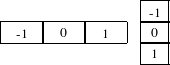
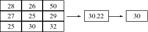
The itk::MeanImageFilter is commonly used for noise reduction. The filter computes the value of each output pixel by finding the statistical mean of the neighborhood of the corresponding input pixel. The following figure illustrates the local effect of the MeanImageFilter. The statistical mean of the neighborhood on the left is passed as the output value associated with the pixel at the center of the neighborhood.
Note that this algorithm is sensitive to the presence of outliers in the neighborhood. This filter will work on images of any dimension thanks to the internal use of itk::SmartNeighborhoodIterator and itk::NeighborhoodOperator . The size of the neighborhood over which the mean is computed can be set by the user.
The header file corresponding to this filter should be included first.
Then the pixel types for input and output image must be defined and, with them, the image types can be instantiated.
Using the image types it is now possible to instantiate the filter type and create the filter object.
The size of the neighborhood is defined along every dimension by passing a SizeType object with the
corresponding values. The value on each dimension is used as the semi-size of a rectangular box. For
example, in 2D a size of  will result in a 3×5 neighborhood.
The input to the filter can be taken from any other filter, for example a reader. The output can be passed down the pipeline to other filters, for example, a writer. An update call on any downstream filter will trigger the execution of the mean filter.
Figure 8.15 illustrates the effect of this filter using neighborhood radii of  which corresponds to a 3×3
classical neighborhood. It can be seen from this picture that edges are rapidly degraded by the diffusion of
intensity values among neighbors.
which corresponds to a 3×3
classical neighborhood. It can be seen from this picture that edges are rapidly degraded by the diffusion of
intensity values among neighbors.
The source code for this example can be found in the file
Examples/Filtering/MedianImageFilter.cxx.
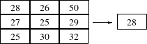
The itk::MedianImageFilter is commonly used as a robust approach for noise reduction. This filter is particularly efficient against salt-and-pepper noise. In other words, it is robust to the presence of gray-level outliers. MedianImageFilter computes the value of each output pixel as the statistical median of the neighborhood of values around the corresponding input pixel. The following figure illustrates the local effect of this filter. The statistical median of the neighborhood on the left is passed as the output value associated with the pixel at the center of the neighborhood.
This filter will work on images of any dimension thanks to the internal use of itk::NeighborhoodIterator and itk::NeighborhoodOperator . The size of the neighborhood over which the median is computed can be set by the user.
The header file corresponding to this filter should be included first.
Then the pixel and image types of the input and output must be defined.
Using the image types, it is now possible to define the filter type and create the filter object.
The size of the neighborhood is defined along every dimension by passing a SizeType object with the
corresponding values. The value on each dimension is used as the semi-size of a rectangular box. For
example, in 2D a size of  will result in a 3×5 neighborhood.
The input to the filter can be taken from any other filter, for example a reader. The output can be passed down the pipeline to other filters, for example, a writer. An update call on any downstream filter will trigger the execution of the median filter.
Figure 8.16 illustrates the effect of the MedianImageFilter filter a neighborhood radius of  , which
corresponds to a 3×3 classical neighborhood. The filtered image demonstrates the moderate tendency of
the median filter to preserve edges.
, which
corresponds to a 3×3 classical neighborhood. The filtered image demonstrates the moderate tendency of
the median filter to preserve edges.
Mathematical morphology has proved to be a powerful resource for image processing and analysis [123]. ITK implements mathematical morphology filters using NeighborhoodIterators and itk::NeighborhoodOperator s. The toolkit contains two types of image morphology algorithms, filters that operate on binary images and filters that operate on grayscale images.
The source code for this example can be found in the file
Examples/Filtering/MathematicalMorphologyBinaryFilters.cxx.
The following section illustrates the use of filters that perform basic mathematical morphology operations on binary images. The itk::BinaryErodeImageFilter and itk::BinaryDilateImageFilter are described here. The filter names clearly specify the type of image on which they operate. The header files required to construct a simple example of the use of the mathematical morphology filters are included below.
The following code defines the input and output pixel types and their associated image types.
Mathematical morphology operations are implemented by applying an operator over the neighborhood of each input pixel. The combination of the rule and the neighborhood is known as structuring element. Although some rules have become de facto standards for image processing, there is a good deal of freedom as to what kind of algorithmic rule should be applied to the neighborhood. The implementation in ITK follows the typical rule of minimum for erosion and maximum for dilation.
The structuring element is implemented as a NeighborhoodOperator. In particular, the default structuring element is the itk::BinaryBallStructuringElement class. This class is instantiated using the pixel type and dimension of the input image.
The structuring element type is then used along with the input and output image types for instantiating the type of the filters.
The filters can now be created by invoking the New() method and assigning the result to itk::SmartPointer s.
The structuring element is not a reference counted class. Thus it is created as a C++ stack object instead of using New() and SmartPointers. The radius of the neighborhood associated with the structuring element is defined with the SetRadius() method and the CreateStructuringElement() method is invoked in order to initialize the operator. The resulting structuring element is passed to the mathematical morphology filter through the SetKernel() method, as illustrated below.
A binary image is provided as input to the filters. This image might be, for example, the output of a binary threshold image filter.
The values that correspond to “objects” in the binary image are specified with the methods SetErodeValue() and SetDilateValue(). The value passed to these methods will be considered the value over which the dilation and erosion rules will apply.
The filter is executed by invoking its Update() method, or by updating any downstream filter, like, for example, an image writer.
Figure 8.17 illustrates the effect of the erosion and dilation filters. The figure shows how these operations can be used to remove spurious details from segmented images.
The source code for this example can be found in the file
Examples/Filtering/MathematicalMorphologyGrayscaleFilters.cxx.
The following section illustrates the use of filters for performing basic mathematical morphology operations on grayscale images. The itk::GrayscaleErodeImageFilter and itk::GrayscaleDilateImageFilter are covered in this example. The filter names clearly specify the type of image on which they operate. The header files required for a simple example of the use of grayscale mathematical morphology filters are presented below.
The following code defines the input and output pixel types and their associated image types.
Mathematical morphology operations are based on the application of an operator over a neighborhood of each input pixel. The combination of the rule and the neighborhood is known as structuring element. Although some rules have become the de facto standard in image processing there is a good deal of freedom as to what kind of algorithmic rule should be applied on the neighborhood. The implementation in ITK follows the typical rule of minimum for erosion and maximum for dilation.
The structuring element is implemented as a itk::NeighborhoodOperator . In particular, the default structuring element is the itk::BinaryBallStructuringElement class. This class is instantiated using the pixel type and dimension of the input image.
The structuring element type is then used along with the input and output image types for instantiating the type of the filters.
The filters can now be created by invoking the New() method and assigning the result to SmartPointers.
The structuring element is not a reference counted class. Thus it is created as a C++ stack object instead of using New() and SmartPointers. The radius of the neighborhood associated with the structuring element is defined with the SetRadius() method and the CreateStructuringElement() method is invoked in order to initialize the operator. The resulting structuring element is passed to the mathematical morphology filter through the SetKernel() method, as illustrated below.
A grayscale image is provided as input to the filters. This image might be, for example, the output of a reader.
The filter is executed by invoking its Update() method, or by updating any downstream filter, like, for example, an image writer.
Figure 8.18 illustrates the effect of the erosion and dilation filters. The figure shows how these operations can be used to remove spurious details from segmented images.
Real image data has a level of uncertainty that is manifested in the variability of measures assigned to pixels. This uncertainty is usually interpreted as noise and considered an undesirable component of the image data. This section describes several methods that can be applied to reduce noise on images.
Blurring is the traditional approach for removing noise from images. It is usually implemented in the form of a convolution with a kernel. The effect of blurring on the image spectrum is to attenuate high spatial frequencies. Different kernels attenuate frequencies in different ways. One of the most commonly used kernels is the Gaussian. Two implementations of Gaussian smoothing are available in the toolkit. The first one is based on a traditional convolution while the other is based on the application of IIR filters that approximate the convolution with a Gaussian [36, 37].
The source code for this example can be found in the file
Examples/Filtering/DiscreteGaussianImageFilter.cxx.
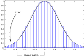
The itk::DiscreteGaussianImageFilter computes the convolution of the input image with a Gaussian kernel. This is done in ND by taking advantage of the separability of the Gaussian kernel. A one-dimensional Gaussian function is discretized on a convolution kernel. The size of the kernel is extended until there are enough discrete points in the Gaussian to ensure that a user-provided maximum error is not exceeded. Since the size of the kernel is unknown a priori, it is necessary to impose a limit to its growth. The user can thus provide a value to be the maximum admissible size of the kernel. Discretization error is defined as the difference between the area under the discrete Gaussian curve (which has finite support) and the area under the continuous Gaussian.
Gaussian kernels in ITK are constructed according to the theory of Tony Lindeberg [88] so that smoothing and derivative operations commute before and after discretization. In other words, finite difference derivatives on an image I that has been smoothed by convolution with the Gaussian are equivalent to finite differences computed on I by convolving with a derivative of the Gaussian.
The first step required to use this filter is to include its header file.
Types should be chosen for the pixels of the input and output images. Image types can be instantiated using the pixel type and dimension.
The discrete Gaussian filter type is instantiated using the input and output image types. A corresponding filter object is created.
The input image can be obtained from the output of another filter. Here, an image reader is used as its input.
The filter requires the user to provide a value for the variance associated with the Gaussian kernel. The method SetVariance() is used for this purpose. The discrete Gaussian is constructed as a convolution kernel. The maximum kernel size can be set by the user. Note that the combination of variance and kernel-size values may result in a truncated Gaussian kernel.
Finally, the filter is executed by invoking the Update() method.
If the output of this filter has been connected to other filters down the pipeline, updating any of the downstream filters would have triggered the execution of this one. For example, a writer could have been used after the filter.
Figure 8.19 illustrates the effect of this filter.
Note that large Gaussian variances will produce large convolution kernels and correspondingly slower computation times. Unless a high degree of accuracy is required, it may be more desirable to use the approximating itk::RecursiveGaussianImageFilter with large variances.
The drawback of image denoising (smoothing) is that it tends to blur away the sharp boundaries in the image that help to distinguish between the larger-scale anatomical structures that one is trying to characterize (which also limits the size of the smoothing kernels in most applications). Even in cases where smoothing does not obliterate boundaries, it tends to distort the fine structure of the image and thereby changes subtle aspects of the anatomical shapes in question.
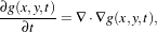
Perona and Malik [106] introduced an alternative to linear-filtering that they called anisotropic diffusion. Anisotropic diffusion is closely related to the earlier work of Grossberg [53], who used similar nonlinear diffusion processes to model human vision. The motivation for anisotropic diffusion (also called nonuniform or variable conductance diffusion) is that a Gaussian smoothed image is a single time slice of the solution to the heat equation, that has the original image as its initial conditions. Thus, the solution to
 | (8.4) |
where g(x,y,0) = f(x,y) is the input image, is g(x,y,t) = G( )⊗f(x,y), where G(σ) is a Gaussian with
standard deviation σ.
)⊗f(x,y), where G(σ) is a Gaussian with
standard deviation σ.
Anisotropic diffusion includes a variable conductance term that, in turn, depends on the differential structure of the image. Thus, the variable conductance can be formulated to limit the smoothing at “edges” in images, as measured by high gradient magnitude, for example.
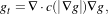 | (8.5) |
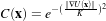
where, for notational convenience, we leave off the independent parameters of g and use the subscripts with respect to those parameters to indicate partial derivatives. The function c(|∇g|) is a fuzzy cutoff that reduces the conductance at areas of large |∇g|, and can be any one of a number of functions. The literature has shown
 | (8.6) |
to be quite effective. Notice that conductance term introduces a free parameter k, the conductance parameter, that controls the sensitivity of the process to edge contrast. Thus, anisotropic diffusion entails two free parameters: the conductance parameter, k, and the time parameter, t, that is analogous to σ, the effective width of the filter when using Gaussian kernels.
Equation 8.5 is a nonlinear partial differential equation that can be solved on a discrete grid using finite forward differences. Thus, the smoothed image is obtained only by an iterative process, not a convolution or non-stationary, linear filter. Typically, the number of iterations required for practical results are small, and large 2D images can be processed in several tens of seconds using carefully written code running on modern, general purpose, single-processor computers. The technique applies readily and effectively to 3D images, but requires more processing time.
In the early 1990’s several research groups [49, 137] demonstrated the effectiveness of anisotropic diffusion on medical images. In a series of papers on the subject [142, 139, 141, 137, 138, 140], Whitaker described a detailed analytical and empirical analysis, introduced a smoothing term in the conductance that made the process more robust, invented a numerical scheme that virtually eliminated directional artifacts in the original algorithm, and generalized anisotropic diffusion to vector-valued images, an image processing technique that can be used on vector-valued medical data (such as the color cryosection data of the Visible Human Project).
For a vector-valued input  : U
: U ℜm the process takes the form
 | (8.7) |
where 
 is a dissimilarity measure of
  , a generalization of the gradient magnitude to vector-valued
images, that can incorporate linear and nonlinear coordinate transformations on the range of
, a generalization of the gradient magnitude to vector-valued
images, that can incorporate linear and nonlinear coordinate transformations on the range of  . In this way,
the smoothing of the multiple images associated with vector-valued data is coupled through the
conductance term, that fuses the information in the different images. Thus vector-valued, nonlinear
diffusion can combine low-level image features (e.g. edges) across all “channels” of a vector-valued image
in order to preserve or enhance those features in all of image “channels”.
. In this way,
the smoothing of the multiple images associated with vector-valued data is coupled through the
conductance term, that fuses the information in the different images. Thus vector-valued, nonlinear
diffusion can combine low-level image features (e.g. edges) across all “channels” of a vector-valued image
in order to preserve or enhance those features in all of image “channels”.
Vector-valued anisotropic diffusion is useful for denoising data from devices that produce multiple values such as MRI or color photography. When performing nonlinear diffusion on a color image, the color channels are diffused separately, but linked through the conductance term. Vector-valued diffusion it is also useful for processing registered data from different devices or for denoising higher-order geometric or statistical features from scalar-valued images [140, 149].
The output of anisotropic diffusion is an image or set of images that demonstrates reduced noise and texture but preserves, and can also enhance, edges. Such images are useful for a variety of processes including statistical classification, visualization, and geometric feature extraction. Previous work has shown [138] that anisotropic diffusion, over a wide range of conductance parameters, offers quantifiable advantages over linear filtering for edge detection in medical images.
Since the effectiveness of nonlinear diffusion was first demonstrated, numerous variations of this approach have surfaced in the literature [128]. These include alternatives for constructing dissimilarity measures [121], directional (i.e., tensor-valued) conductance terms [135, 6] and level set interpretations [143].
The source code for this example can be found in the file
Examples/Filtering/GradientAnisotropicDiffusionImageFilter.cxx.
The itk::GradientAnisotropicDiffusionImageFilter implements an N-dimensional version of the classic Perona-Malik anisotropic diffusion equation for scalar-valued images [106].
The conductance term for this implementation is chosen as a function of the gradient magnitude of the image at each point, reducing the strength of diffusion at edge pixels.
 | (8.8) |
The numerical implementation of this equation is similar to that described in the Perona-Malik paper [106], but uses a more robust technique for gradient magnitude estimation and has been generalized to N-dimensions.
The first step required to use this filter is to include its header file.
Types should be selected based on the pixel types required for the input and output images. The image types are defined using the pixel type and the dimension.
The filter type is now instantiated using both the input image and the output image types. The filter object is created by the New() method.
The input image can be obtained from the output of another filter. Here, an image reader is used as source.
This filter requires three parameters, the number of iterations to be performed, the time step and the conductance parameter used in the computation of the level set evolution. These parameters are set using the methods SetNumberOfIterations(), SetTimeStep() and SetConductanceParameter() respectively. The filter can be executed by invoking Update().
A typical value for the time step is 0.125. The number of iterations is typically set to 5; more iterations result in further smoothing and will increase the computing time linearly.
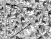
Figure 8.20 illustrates the effect of this filter. In this example the filter was run with a time step of 0.125, and 5 iterations. The figure shows how homogeneous regions are smoothed and edges are preserved.
The following classes provide similar functionality:
The source code for this example can be found in the file
Examples/BasicFilters/MeanShiftSegmentationFilterExample.cxx.
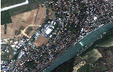
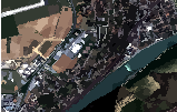
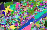
This example demonstrates the use of the otb::MeanShiftSegmentationFilter class which implements filtering and clustering using the mean shift algorithm [29]. For a given pixel, the mean shift will build a set of neighboring pixels within a given spatial radius and a color range. The spatial and color center of this set is then computed and the algorithm iterates with this new spatial and color center. The Mean Shift can be used for edge-preserving smoothing, or for clustering.
We start by including the needed header file.
We start by the classical typedefs needed for reading and writing the images.
We instantiate the filter, the reader, and 2 writers (for the labeled and clustered images).
We set the file names for the reader and the writers:
We can now set the parameters for the filter. There are 3 main parameters: the spatial radius used for defining the neighborhood, the range radius used for defining the interval in the color space and the minimum size for the regions to be kept after clustering.
Two another parameters can be set : the maximum iteration number, which defines maximum number of iteration until convergence. Algorithm iterative scheme will stop if convergence hasn’t been reached after the maximum number of iterations. Threshold parameter defines mean-shift vector convergence value. Algorithm iterative scheme will stop if mean-shift vector is below this threshold or if iteration number reached maximum number of iterations.
We can now plug the pipeline and run it.
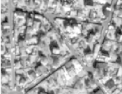
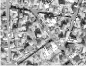
Figure 8.21 shows the result of applying the mean shift to a Quickbird image.
The source code for this example can be found in the file
Examples/BasicFilters/LeeImageFilter.cxx.
This example illustrates the use of the otb::LeeImageFilter . This filter belongs to the family of the edge-preserving smoothing filters which are usually used for speckle reduction in radar images. The Lee filter [85] aplies a linear regression which minimizes the mean-square error in the frame of a multiplicative speckle model.
The first step required to use this filter is to include its header file.
Then we must decide what pixel type to use for the image.
The images are defined using the pixel type and the dimension.
The filter can be instantiated using the image types defined above.
An otb::ImageFileReader class is also instantiated in order to read image data from a file.
An otb::ImageFileWriter is instantiated in order to write the output image to a file.
Both the filter and the reader are created by invoking their New() methods and assigning the result to SmartPointers.
The image obtained with the reader is passed as input to the otb::LeeImageFilter .
The method SetRadius() defines the size of the window to be used for the computation of the local statistics. The method SetNbLooks() sets the number of looks of the input image.
Figure 8.22 shows the result of applying the Lee filter to a SAR image.
The following classes provide similar functionality:
The source code for this example can be found in the file
Examples/BasicFilters/FrostImageFilter.cxx.
This example illustrates the use of the otb::FrostImageFilter . This filter belongs to the family of the edge-preserving smoothing filters which are usually used for speckle reduction in radar images.
This filter uses a negative exponential convolution kernel. The output of the filter for pixel p is: Îs = ∑p∈ηpmpIp
where : mp = 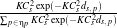 and ds,p =
Most of this example is similar to the previous one and only the differences will be highlighted.
First, we need to include the header:
The filter can be instantiated using the image types defined previously.
The image obtained with the reader is passed as input to the otb::FrostImageFilter .
The method SetRadius() defines the size of the window to be used for the computation of the local statistics. The method SetDeramp() sets the K coefficient.
Figure 8.23 shows the result of applying the Frost filter to a SAR image.
The following classes provide similar functionality:
The Markov Random Field framework for OTB is more detailed in 19.4.6.2 (p. 865).
The source code for this example can be found in the file
Examples/Markov/MarkovRestorationExample.cxx.
The Markov Random Field framework can be used to apply an edge preserving filtering, thus playing a role of restoration.
This example applies the otb::MarkovRandomFieldFilter for image restoration. The structure of the example is similar to the other MRF example. The original image is assumed to be coded in one byte, thus 256 states are possible for each pixel. The only other modifications reside in the energy function chosen for the fidelity and for the regularization.
For the regularization energy function, we choose an edge preserving function:
 | (8.9) |
and for the fidelity function, we choose a gaussian model.
The starting state of the Markov Random Field is given by the image itself as the final state should not be too far from it.
The first step toward the use of this filter is the inclusion of the proper header files:
We declare the usual types:
We need to declare an additional reader for the initial state of the MRF. This reader has to be instantiated on the LabelledImageType.
We declare all the necessary types for the MRF:
The regularization and the fidelity energy are declared and instantiated:
The number of possible states for each pixel is 256 as the image is assumed to be coded on one byte and we pass the parameters to the markovFilter.
The original state of the MRF filter is passed through the SetTrainingInput() method:
And we plug the pipeline:
Figure 8.24 shows the output of the Markov Random Field restoration.


The source code for this example can be found in the file
Examples/Filtering/DanielssonDistanceMapImageFilter.cxx.
This example illustrates the use of the itk::DanielssonDistanceMapImageFilter . This filter generates a distance map from the input image using the algorithm developed by Danielsson [32]. As secondary outputs, a Voronoi partition of the input elements is produced, as well as a vector image with the components of the distance vector to the closest point. The input to the map is assumed to be a set of points on the input image. Each point/pixel is considered to be a separate entity even if they share the same gray level value.
The first step required to use this filter is to include its header file.
Then we must decide what pixel types to use for the input and output images. Since the output will contain distances measured in pixels, the pixel type should be able to represent at least the width of the image, or said in N -D terms, the maximum extension along all the dimensions. The input and output image types are now defined using their respective pixel type and dimension.
The filter type can be instantiated using the input and output image types defined above. A filter object is created with the New() method.
The input to the filter is taken from a reader and its output is passed to a itk::RescaleIntensityImageFilter and then to a writer.
The type of input image has to be specified. In this case, a binary image is selected.
Figure 8.25 illustrates the effect of this filter on a binary image with a set of points. The input image is shown at left, the distance map at the center and the Voronoi partition at right. This filter computes distance maps in N-dimensions and is therefore capable of producing N -D Voronoi partitions.
The Voronoi map is obtained with the GetVoronoiMap() method. In the lines below we connect this output to the intensity rescaler and save the result in a file.
Execution of the writer is triggered by the invocation of the Update() method. Since this method can potentially throw exceptions it must be placed in a try/catch block.