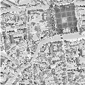
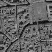
Figure 23.1: On the left, the image obtained by truncated pixel values at the dynamic acceptable for a png file
(between 0 and 255). On the right, the same image with a proper rescaling
After processing your images with OTB, you probably want to see the result. As it is quite straightforward in some situation, if can be a bit trickier in other. For example, some filters will give you a list of polygons as an output. Other can return an image with each region labelled by a unique index. In this section we are going to provide few examples to help you produce beautiful output ready to be included in your publications/presentations.
The source code for this example can be found in the file
On one hand, satellite images are commonly coded on more than 8 bits to provide the dynamic range required from shadows to clouds. On the other hand, image formats in use for printing and display are usually limited to 8 bits. We need to convert the value to enable a proper display. This is usually done using linear scaling. Of course, you have to be aware that some information is lost in the process.
The
Figure 23.1 illustrates the difference between a proper scaling and a simple truncation of the value and demonstrates why it is important to keep this in mind.
The source code for this example can be found in the file
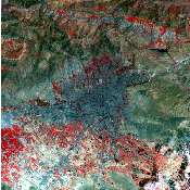
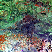
Most of the time, satellite images have more than three spectral bands. As we are only able to see three colors (red, green and blue), we have to find a way to represent these images using only three bands. This is called creating a color composition.
Of course, any color composition will not be able to render all the information available in the original image. As a consequence, sometimes, creating more than one color composition will be necessary.
If you want to obtain an image with natural colors, you have to match the wavelength captured by the satellite with those captured by your eye: thus matching the red band with the red color, etc.
Some satellites (SPOT 5 is an example) do not acquire all the
The band order in the image products can be also quite tricky. It could be in the wavelength order, as it is the case for Quickbird (1: Blue, 2: Green, 3: Red, 4: NIR), in this case, you have to be careful to reverse the order if you want a natural display. It could also be reverse to facilitate direct viewing, as for SPOT5 (1: NIR, 2: Red, 3: Green, 4: SWIR) but in this situations you have to be careful when you process the image.
To easily convert the image to a
When you create the writer to plug at the output of the
Figure 23.2 illustrates different color compositions for a SPOT 5 image.
The source code for this example can be found in the file
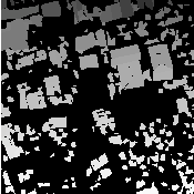
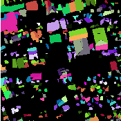
Some algorithms produce an indexed image as output. In such images, each pixel is given a value according to the region number it belongs to. This value starting at 0 or 1 is usually an integer value. Often, such images are produced by segmentation or classification algorithms.
If such regions are easy to manipulate – it is easier and faster to compare two integers than a RGB value – it is different when it comes to displaying the results.
Here we present a convient way to convert such indexed image to a color image. In such conversion, it is
important to ensure that neighborhood region, which are likely to have consecutive number have easily
dicernable colors. This is done randomly using a hash function by the
The
Figure 23.3 shows the result of the conversion from an indexed image to a color image.
The source code for this example can be found in the file
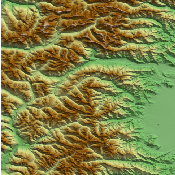
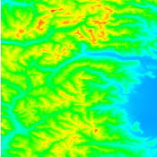
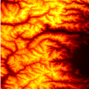
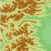
In some situation, it is desirable to represent a gray scale image in color for easier interpretation. This is particularly the case if pixel values in the image are used to represent some data such as elevation, deformation map, interferogram. In this case, it is important to ensure that similar values will get similar colors. You can notice how this requirement differs from the previous case.
The following example illustrates the use of the
As in the previous example, the
And we connect the color mapper filter with the filter producing the image of the DEM:
Figure 23.4 shows the effect of applying the filter to a gray scale image.
The source code for this example can be found in the file
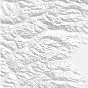
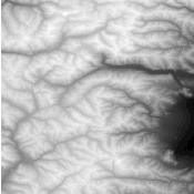
Visualization of digital elevation models (DEM) is often more intuitive by simulating a lighting source and generating the corresponding shadows. This principle is called hill shading.
Using a simple functor
This example will focus on the shading itself.
After generating the DEM image as in the DEMToImageGenerator example, you can declare the hill
shading mechanism. The hill shading is implemented as a functor doing some operations in its
neighborhood. A convenient filter called
Figure 23.5 shows the hill shading result from SRTM data.